leapR
leapR.RmdInstallation
This is intended to be a short introduction to the leapR
package. First we need to load the required libraries:
# install from bioconductor
if (!require(BiocManager)) {
  install.packages('BiocManager')
  BiocManager::install('leapR')
}Introduction
Definitions
Dataset - an expression dataset, contained in the Bioconductor object, that at the bare minimum has a matrix of components (rows) measured in the same system under multiple different conditions (columns)
Component - the things being measured, genes, proteins, methylation site, phosphosite, etc. For functional (currently) the component must be associated with a gene name. That is, there’s not currently a way to calculate pathway enrichment using lipids.
Pathway - a set of components that works together to accomplish something or are related to each other in some other way. This includes classic signaling and metabolic pathways, but also molecular function and localization categories and other groups of related components, like genome location, conservation, etc.
Condition - a sample where the treatment, environmental conditions, patient, time point or some combination of those is varied.
The overall idea for functional enrichment is to determine which pathways are statistically over-represented in one group versus another, display statistically differential abundance from one group to another, or are statistically differentially distributed in a ranked list based on the abundance of one sample. Each of these purposes has a different underlying statistical test (or family of tests) and the results of each can be interpreted in somewhat different ways. The purpose of this vignette is to give the user a very brief introduction on how to use the package, not to discuss the underlying statistical choices that need to be made when analyzing such data.
There are a number of caveats (probably non-exhaustive) with doing this kind of analysis.
Important points for consideration
Data normalization
One important point is to use data that’s been normalized in a particular way to do these analyses. Data here has been normalized as a Z score by row (gene/protein/etc.). So, for each row, calculate the mean and standard deviation across all the conditions (columns) and then express as a Z score.
Here’s why. All high-throughput technologies (microarray, RNAseq, MS-assisted proteomics, metabolomics, lipidomics, etc.) suffer from the same limitation. The detectability of each molecule being detected (protein, RNA, etc.) is different and, in general, it’s impossible to accurately determine how detectable each one is. The multi-omic functional enrichment process lumps together measurements from different components (proteins, genes, etc.) to summarize a pathway. If the component measurements aren’t directly comparable (they aren’t) then this can and will introduce significant systematic errors and won’t produce the results you’re looking for. Careful consideration must be given that the results of the analysis reflect the question being asked and that the normalization method hasn’t obscured the desired results.
Background
The background of comparison for functional enrichment is always important, but it mainly impacts the Fisher’s exact tests in the examples below. The background answers the question: “My functional group of interest is statistically enriched relative to what?” For Fisher’s exact tests this is critical. Generally, it is best to compare enrichment against the components observed in the data (the experiment’s universe) rather than the universe of all possible components. For example, a proteomics dataset from plasma may contain a limited set of proteins compared with all possible human proteins; using the observed proteins as the background usually yields more meaningful results. Using all possible proteins will result in substantially different findings.
Multiple hypothesis correction
When testing the statistical significance of differences in a lot of pathways it’s necessary to correct for multiple hypotheses. This essentially accounts for the possibility you might see SOMETHING significant by chance if you just test enough things- so it moves p values in a less significant direction. The more things you test, the greater this move will be. So pathway databases with lots of pathways are affected more by this correction, making it harder to get a significant result (which is a good thing actually).
Pathway databases
Two ‘databases’ (organized text files) are included for pathways. The example is taken from the NCI’s Pathway Interaction Database (PID) and covers signaling pathways in human - but is no longer being actively maintained. They can be loaded as follows:
data(ncipid)Identifiers
The identifiers (gene names, e.g.) for the data input MUST match the identifiers used in the pathway database. The two included human databases use the HGNC-approved gene names. Which means your data has to use the same identifiers.
Example data
A sample data set is included that is from the CPTAC study of 169
ovarian tumors. We include the dataset as a object, containing three
assays (transcriptomics, global proteomics, and phosphoproteomics) to
enable interoperability with other tools, and store example file as
rda on Figshare
as example.
This data can be loaded as follows:
# Inspect the `pset` SummarizedExperiment.
str(pset)
#> Formal class 'SummarizedExperiment' [package "SummarizedExperiment"] with 5 slots
#>   ..@ colData        :Formal class 'DFrame' [package "S4Vectors"] with 6 slots
#>   .. .. ..@ rownames       : chr [1:174] "TCGA-09-1664" "TCGA-09-2056" "TCGA-13-1404" "TCGA-13-1409" ...
#>   .. .. ..@ nrows          : int 174
#>   .. .. ..@ elementType    : chr "ANY"
#>   .. .. ..@ elementMetadata: NULL
#>   .. .. ..@ metadata       : list()
#>   .. .. ..@ listData       : Named list()
#>   ..@ assays         :Formal class 'SimpleAssays' [package "SummarizedExperiment"] with 1 slot
#>   .. .. ..@ data:Formal class 'SimpleList' [package "S4Vectors"] with 4 slots
#>   .. .. .. .. ..@ listData       :List of 1
#>   .. .. .. .. .. ..$ proteomics: num [1:18632, 1:174] -4.0649 -0.1398 -0.0366 0.768 0.2437 ...
#>   .. .. .. .. .. .. ..- attr(*, "dimnames")=List of 2
#>   .. .. .. .. .. .. .. ..$ : chr [1:18632] "C9orf152" "ELMO2" "RPS11" "CREB3L1" ...
#>   .. .. .. .. .. .. .. ..$ : chr [1:174] "TCGA-09-1664" "TCGA-09-2056" "TCGA-13-1404" "TCGA-13-1409" ...
#>   .. .. .. .. ..@ elementType    : chr "ANY"
#>   .. .. .. .. ..@ elementMetadata: NULL
#>   .. .. .. .. ..@ metadata       : list()
#>   ..@ NAMES          : chr [1:18632] "C9orf152" "ELMO2" "RPS11" "CREB3L1" ...
#>   ..@ elementMetadata:Formal class 'DFrame' [package "S4Vectors"] with 6 slots
#>   .. .. ..@ rownames       : NULL
#>   .. .. ..@ nrows          : int 18632
#>   .. .. ..@ elementType    : chr "ANY"
#>   .. .. ..@ elementMetadata: NULL
#>   .. .. ..@ metadata       : list()
#>   .. .. ..@ listData       : Named list()
#>   ..@ metadata       : list()
dim(SummarizedExperiment::assay(pset, "proteomics"))
#> [1] 18632   174
head(rownames(pset))
#> [1] "C9orf152" "ELMO2"    "RPS11"    "CREB3L1"  "PNMA1"    "MMP2"
head(colnames(pset))
#> [1] "TCGA-09-1664" "TCGA-09-2056" "TCGA-13-1404" "TCGA-13-1409" "TCGA-13-1410"
#> [6] "TCGA-13-1482"
We also include some groups of patients to compare stored as R data objects:
data(shortlist)
data(longlist)

## columns that we want to use for results

cols_to_display <- c("ingroup_n", "outgroup_n", "background_n",
                     "pvalue", "BH_pvalue")
The data are now loaded and ready to go through some of the examples.
Examples
We include five examples of how to use this tool, depending on the analysis at hand. ## Comparison of one condition/group versus another condition/group.
There are a number of ways to do this. I generally use a simple approach which assesses the statistical difference in distributions between the abundance values from all the members of a pathway in all the group members from one group with those from the other group using a t test.
Caveat
This is a ‘bag of values’ approach and it does not pay attention to the relationships between values in different groups (i.e. that each group has measurements for the same component). There are likely issues that rise because of this and caveats associated with it. However, it works fairly well.
Description
In this example we are assessing the enrichment of pathways in a
group of short surviving patients versus in a group of long
surviving
patients. We can also do a single patient-to-patient comparison or
compare a single patient to a group of patients.
Interpretation
Better corrected p-values are more enriched. However, you can get
good p-values when the algorithm only considers a limited number of
components from a pathway. That is, the pathway may have 30 members and
the p-value is coming from values from just 3 members. You can look at
the ingroup_n column from the result matrix to see this
(and screen out if desired).
It is VERY important to also consider the effect size. That is, the
difference between the mean of one group and the mean of the other
group. If there are large numbers of components in the pathway being
compared it is relatively easy to get a significant p value with small
effect size. Though this may be a real difference it is often not as
interesting as a smaller group with worse p value and greater effect
size. You can look at the effect size by comparing the
ingroup_mean and outgroup_mean columns.
# in this example we lump a bunch of patients together (the 'short survivors')
# and compare them to another group (the 'long survivors')

### using enrichment_wrapper function
protdata.enrichment.svl <- leapR::leapR(
  geneset = ncipid,
  enrichment_method = "enrichment_comparison",
  eset = pset,
  assay_name = "proteomics",
  primary_columns = shortlist,
  secondary_columns = longlist
)

or <- order(unlist(protdata.enrichment.svl[, "pvalue"]))
rmarkdown::paged_table(protdata.enrichment.svl[or, cols_to_display])
# another application is to compare just one patient against another
# (this would be the  equivalent of comparing one time point to another)

### using enrichment_wrapper function
protdata.enrichment.svl.ovo <- leapR::leapR(
  geneset = ncipid,
  enrichment_method = "enrichment_comparison",
  eset = pset,
  assay_name = "proteomics",
  primary_columns = shortlist[1],
  secondary_columns = longlist[1]
)
or <- order(unlist(protdata.enrichment.svl.ovo[, "pvalue"]))
rmarkdown::paged_table(protdata.enrichment.svl.ovo[or, cols_to_display])
When we only compare one sample to another, we get no enriched pathways.
Fisher’s exact test
For this test I use Fisher’s exact which is a simple comparison of the overlap of two sets (think of it like a statistical Venn diagram with two groups). It’s also referred to as a hypergeometric test.
Caveats
Caveat 1. Fisher’s exact does not consider abundance values but only lists of components. Generally this requires some separation of a group of interest using differential expression, module membership (from a network for example), or some other method.
Caveat 2. The choice of background for comparison can make a big difference on outcome. For example, in a proteomics experiment where you’re looking at enrichment in a group of highly differentially expressed proteins, you could choose to use all possible proteins as a background, or you could use just those proteins that were observed by proteomics (generally a much more limited set). The second option is generally the best since the first options will result in (partly to mostly) functions that are enriched in proteins that are seen in proteomics. That is, the most abundant proteins, which is generally not the desired outcome.
Description
In the example below I construct a genelist of interest using a simple abundance threshold on the data then use a background of all the genes in the example dataset (which is a limited number). I then do a simple hierarchical clustering on the data, extract modules, and step through each module to calculate enrichment for them, outputting the results into a separate text file.
Interpretation
As with the t test comparison above it is important to look at the number of pathway members included in the comparison (look at the in_path column). There is no ‘effect size’ problem with Fisher’s exact since it’s just a set comparison, but it’s important to note that significant p values can arise from a pathway being underrepresented in the genelist, which often times is not the desired result. The foldx column gives a ratio of in versus not in the genelist, values > 1 being enriched and <1 being depleted.
# for this example we will construct a list of genes from the expression data
#     to emulate what you might be inputting
genelist <- rownames(pset)[which(SummarizedExperiment::assay(pset,
                                                    "proteomics")[, 1] > 0.5)]

protdata.enrichment.sets.test <- leapR::leapR(
  geneset = ncipid,
  enrichment_method = "enrichment_in_sets",
  eset = pset,
  assay_name = "proteomics",
  targets = genelist
)
or <- order(protdata.enrichment.sets.test[, "pvalue"])
rmarkdown::paged_table(protdata.enrichment.sets.test[or, cols_to_display])
# in this example we construct some modules from the hierarchical clustering
#   of the   data
protdata_naf <- SummarizedExperiment::assay(pset, "proteomics")

# hierarchical clustering is not too happy with lots of missing values
#    so we'll do a zero fill on this to get the modules
protdata_naf[which(is.na(protdata_naf))] <- 0

# construct the hierarchical clustering using the 'wardD' method, which
#    seems to give more even sized modules
protdata_hc <- hclust(dist(protdata_naf), method = "ward.D2")

# arbitrarily we'll chop the clusters into 5 modules
modules <- cutree(protdata_hc, k = 5)

## sara: created list
clusters <- lapply(unique(modules), function(x) names(which(modules == x)))

# modules is a named list of values where each value is a module
#         number and the name is the gene name

# To do enrichment for one module (module 1 in this case) do this
protdata.enrichment.sets.module_1 <- leapR::leapR(
  geneset = ncipid,
  enrichment_method = "enrichment_in_sets",
  eset = pset,
  assay_name = "proteomics",
  targets = names(modules[which(modules == 1)])
)

# To do enrichment on all modules and return the list of enrichment results
protdata.enrichment.sets.modules <- do.call(rbind,
                                            leapR::cluster_enrichment(
                                                eset = pset,
                                                assay_name= 'proteomics',
                                                geneset = ncipid,
                                                clusters = clusters,
                                                sigfilter = 0.25))
## nothing is enriched
rmarkdown::paged_table(protdata.enrichment.sets.modules[, cols_to_display])
Visualizing Fisher’s exact results
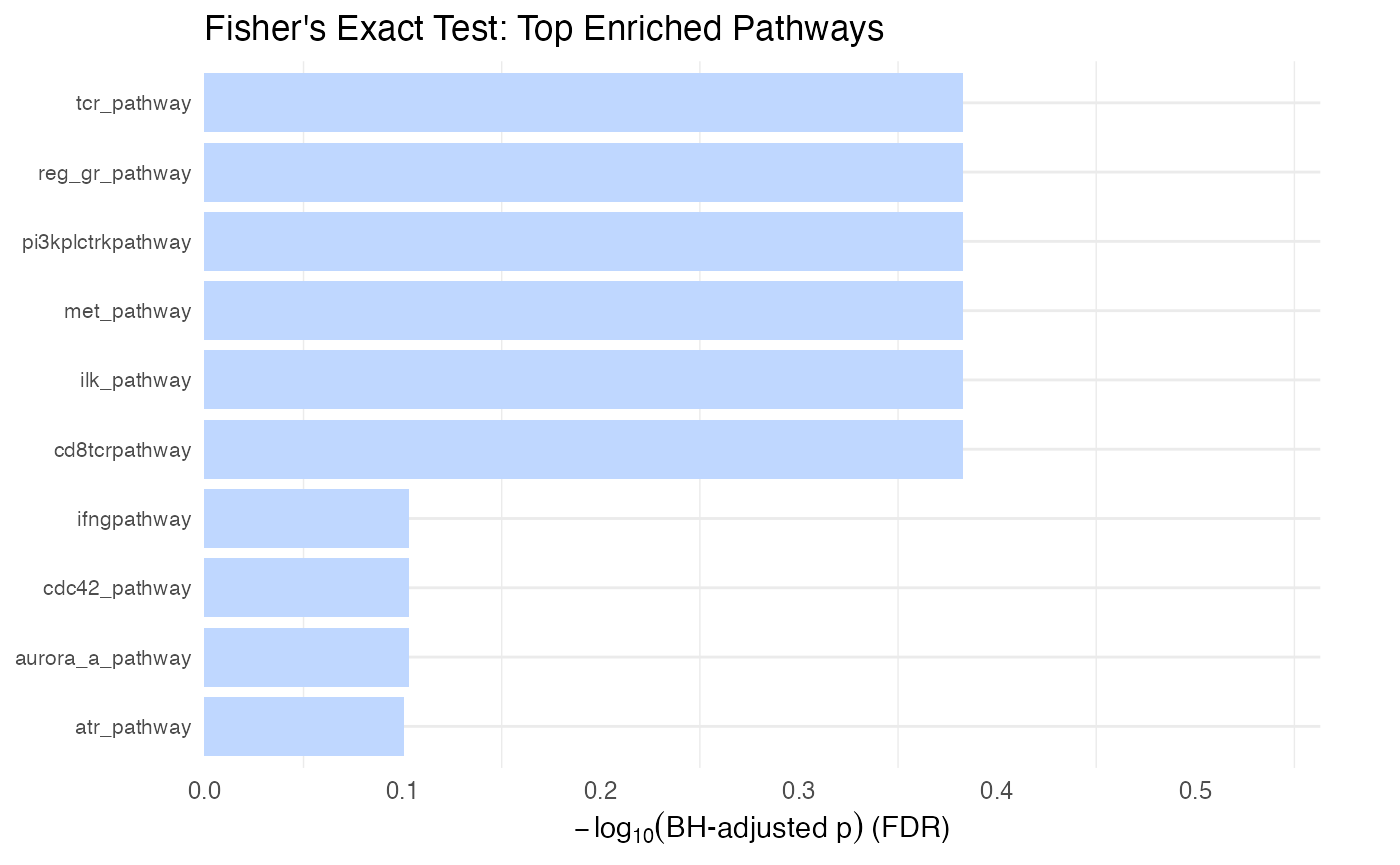
# Plot the top enriched gene sets from Fisher's exact test
# Stars indicate significance (None seen here)
plot_leapr_bar(
  protdata.enrichment.sets.test,
  title = "Fisher's Exact Test: Top Enriched Pathways",
  top_n = 10,
  star_thresholds = c(0.05, 0.01, 0.001),
  wrap = 40
)
The Kolmogorov–Smirnov test (KS)
Similar to the popular GSEA, KS tests whether a group of components (the pathway) is distributed in a statistically significant manner in a ranked list of components. That is, if all the members of the pathway are clustered together at the top of the list (highly abundant, e.g.) or at the bottom of the list (low abundance, e.g.) this will return good p values. I should note that GSEA uses a more sophisticated approach than this and their application has a lot of bells and whistles.
Description
In the example below I’m simply calculating enrichment for one of the patients in the list (arbitrarily selected). The ranking value is relative protein abundance in this case, but can be any continuous measure or derived value. For example, you could calculate the topology of all proteins in a network and use the topology measure (degree) as the measure.
Interpretation
Similar to the other examples be cautious of pathways with good p values that consider a small number of pathway numbers (in_path column). The MeanPath column gives a measure that shows how far above or below the median the mean rank of the pathway is (normalized to -1,1). The Zscore column is a Zscore calculated on the basis of the mean percentage rank of the pathway relative to the mean of the entire list divided by the standard deviation of the pathway rank. The foldx column expresses the mean percentage rank of the pathway relative to the entire list - closer to 0 is higher in the list and closer to 1 is closer to the bottom of the list. Each of these should give consistent results, but will be somewhat different.
# This is how you calculate enrichment in a ranked list
# (for example from topology)
### using enrichment_wrapper function
protdata.enrichment.order <- leapR::leapR(
geneset = ncipid, "enrichment_in_order",
eset = pset,
method = 'ks',
assay_name = "proteomics",
primary_columns = shortlist[1]
)
or <- order(protdata.enrichment.order[, "pvalue"])
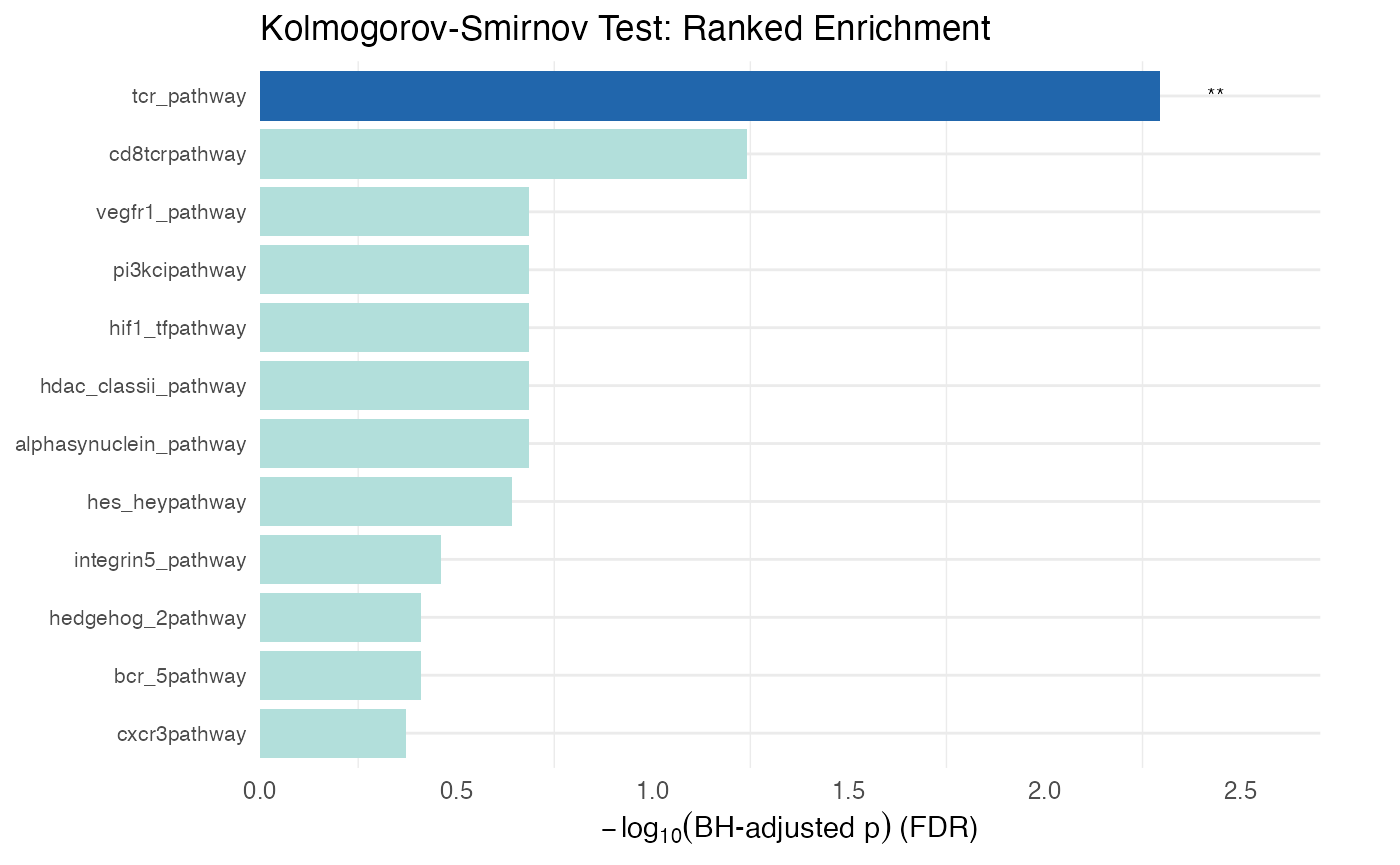
rmarkdown::paged_table(protdata.enrichment.order[or, cols_to_display])Visualizing KS test results
# Plot the ranked enrichment results
plot_leapr_bar(
  protdata.enrichment.order,
  title = "Kolmogorov-Smirnov Test: Ranked Enrichment",
  top_n = 12,
  fill_sig = "#2166AC",
  fill_ns = "#B2DFDB",
  wrap = 38
)
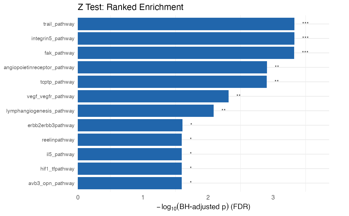
KS alternative: the one-sample Z test
Given that the KS test has not always been the best for gene set enrichment we also implement the one-sample z test.
# This is how you calculate enrichment in a ranked list
# (for example from topology)
### using enrichment_wrapper function
protdata.enrichment.order <- leapR::leapR(
  geneset = ncipid, "enrichment_in_order",
  eset = pset,
  method = 'ztest',
  assay_name = "proteomics",
  primary_columns = shortlist[1]
)


or <- order(protdata.enrichment.order[, "pvalue"])
rmarkdown::paged_table(protdata.enrichment.order[or, cols_to_display])
plot_leapr_bar(
  protdata.enrichment.order,
  title = "Z Test: Ranked Enrichment",
  top_n = 12,
  fill_sig = "#2166AC",
  fill_ns = "#B2DFDB",
  wrap = 38
)
Enrichment in Correlation
The idea here is to use the correlation of pathway members to each other versus to non-pathway members as a way to assess functional enrichment. This idea seems sound- pathways that are varying in a correlated way across a bunch of conditions (say time points or patients) may be more active and more important than others. However, more testing and validation is needed to show that this is the case.
Interpretation
The ingroup_mean gives the mean correlation of the
pathway members to each other and outgroup_mean gives the correlation of
the pathway members to non-pathway members. Background_mean gives the
mean correlation of all non-pathway members. The pvalue and
BH_pvalue are for the pathway members to each other versus
those pathway members to non-pathway components. The
pvalue_background and BH_pvalue_background are
for the pathway member correlation relative to non-pathway member
correlation (which is similar but slightly different than the other
p-values).
### using enrichment_wrapper function
protdata.enrichment.correlation <- leapR::leapR(
  geneset = ncipid,
  enrichment_method = "correlation_enrichment",
  assay_name = "proteomics",
  eset = pset
)

or <- order(protdata.enrichment.correlation[, "pvalue"])
rmarkdown::paged_table(head(protdata.enrichment.correlation[or,
                                                      cols_to_display]))
protdata.enrichment.correlation.short <- leapR::leapR(
  geneset = ncipid,
  enrichment_method = "correlation_enrichment",
  assay_name = "proteomics",
  eset = pset[, shortlist]
)
or <- order(protdata.enrichment.correlation.short[, "pvalue"])
rmarkdown::paged_table(head(protdata.enrichment.correlation.short[or,
                                                        cols_to_display]))
protdata.enrichment.correlation.long <- leapR::leapR(
geneset = ncipid,
enrichment_method = "correlation_enrichment",
assay_name = "proteomics",
eset = pset[, longlist]
)
or <- order(protdata.enrichment.correlation.long[, "pvalue"])
rmarkdown::paged_table(head(protdata.enrichment.correlation.long[or,
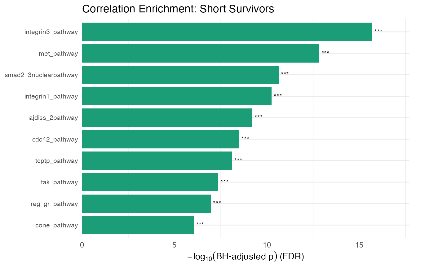
cols_to_display]))Visualizing correlation enrichment results
# Compare correlation patterns across conditions
plot_leapr_bar(
  protdata.enrichment.correlation.short,
  title = "Correlation Enrichment: Short Survivors",
  top_n = 10,
  fill_sig = "#1B9E77",
  fill_ns = "#D8F0E8",
  wrap = 36
)
Phosphoproteomics data analysis
In this example we will use phosphoproteomics data to assess the enrichment in known kinase substrates (a proxy for kinase activity)
data("kinasesubstrates")

# for an individual tumor calculate the Kinase-Substrate
# Enrichment (similar to KSEA)
#     This uses the site-specific phosphorylation data to determine
# which kinases
#     might be active by assessing the enrichment of the
# phosphorylation of their known substrates

phosphodata.ksea.order <- leapR::leapR(
  geneset = kinasesubstrates,
  enrichment_method = "enrichment_in_order",
  assay_name = "phosphoproteomics",
  eset = phset,
  method = 'ztest',
  primary_columns = "TCGA-13-1484")

or <- order(phosphodata.ksea.order[, "pvalue"])
rmarkdown::paged_table(phosphodata.ksea.order[or, cols_to_display])
# now do the same thing but use a threshold
phosphodata.sets.order <- leapR::leapR(
  geneset = kinasesubstrates,
  enrichment_method = "enrichment_in_sets",
  eset = phset,
  assay_name = "phosphoproteomics",
  threshold = 0.5,
  primary_columns = "TCGA-13-1484"
)
or <- order(phosphodata.sets.order[, "pvalue"])
rmarkdown::paged_table(phosphodata.sets.order[or, cols_to_display])
Visualizing kinase substrate enrichment
plot <- plot_leapr_bar(
  phosphodata.sets.order,
  title            = "Kinase Substrate Enrichment (Phosphoproteomics)",
  top_n            = 15,
  star_thresholds  = c(0.05, 0.01, 1e-3),
  wrap             = 36,
  fill_sig         = "#0F766E",  # dark teal for significant
  fill_ns          = "#99F6E4",  # light teal for non-significant
  outline          = "grey30",
  axis_text_y_size = 7,
  axis_text_x_size = 8
)

plot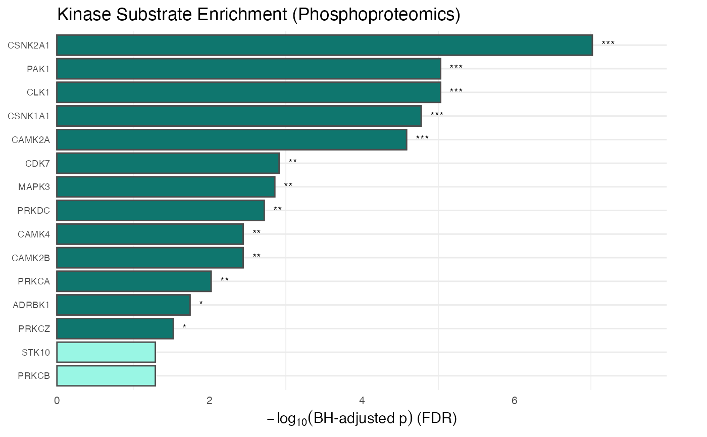
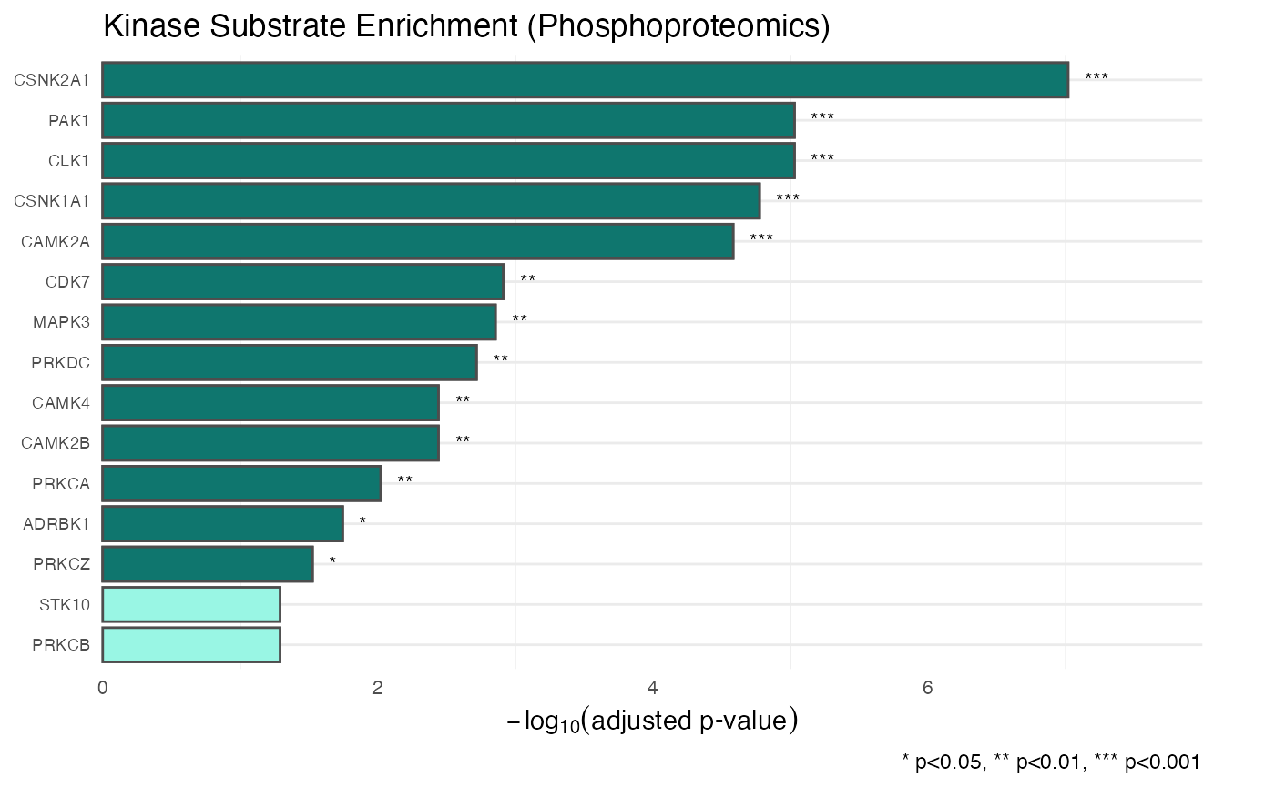
# You can also modify the plot further using standard ggplot2 arguments
plot + ggplot2::labs(
  y = expression(-log[10]("adjusted p-value")),
  caption = "* p<0.05, ** p<0.01, *** p<0.001"
)
Lastly we print out the session info!
sessionInfo()
#> R version 4.6.0 (2026-04-24)
#> Platform: x86_64-pc-linux-gnu
#> Running under: Ubuntu 24.04.4 LTS
#>
#> Matrix products: default
#> BLAS:   /usr/lib/x86_64-linux-gnu/openblas-pthread/libblas.so.3
#> LAPACK: /usr/lib/x86_64-linux-gnu/openblas-pthread/libopenblasp-r0.3.26.so;  LAPACK version 3.12.0
#>
#> locale:
#>  [1] LC_CTYPE=C.UTF-8       LC_NUMERIC=C           LC_TIME=C.UTF-8
#>  [4] LC_COLLATE=C.UTF-8     LC_MONETARY=C.UTF-8    LC_MESSAGES=C.UTF-8
#>  [7] LC_PAPER=C.UTF-8       LC_NAME=C              LC_ADDRESS=C
#> [10] LC_TELEPHONE=C         LC_MEASUREMENT=C.UTF-8 LC_IDENTIFICATION=C
#>
#> time zone: UTC
#> tzcode source: system (glibc)
#>
#> attached base packages:
#> [1] stats     graphics  grDevices utils     datasets  methods   base
#>
#> other attached packages:
#>  [1] BiocFileCache_3.2.0 dbplyr_2.5.2        stringr_1.6.0
#>  [4] tibble_3.3.1        dplyr_1.2.1         ggplot2_4.0.3
#>  [7] rmarkdown_2.31      gplots_3.3.0        leapR_1.1.2
#> [10] BiocStyle_2.40.0
#>
#> loaded via a namespace (and not attached):
#>  [1] SummarizedExperiment_1.42.0 gtable_0.3.6
#>  [3] httr2_1.2.2                 xfun_0.58
#>  [5] bslib_0.11.0                caTools_1.18.3
#>  [7] Biobase_2.72.0              lattice_0.22-9
#>  [9] tzdb_0.5.0                  vctrs_0.7.3
#> [11] tools_4.6.0                 bitops_1.0-9
#> [13] generics_0.1.4              curl_7.1.0
#> [15] stats4_4.6.0                RSQLite_3.53.1
#> [17] blob_1.3.0                  pkgconfig_2.0.3
#> [19] Matrix_1.7-5                KernSmooth_2.23-26
#> [21] RColorBrewer_1.1-3          S7_0.2.2
#> [23] desc_1.4.3                  S4Vectors_0.50.1
#> [25] lifecycle_1.0.5             compiler_4.6.0
#> [27] farver_2.1.2                textshaping_1.0.5
#> [29] Seqinfo_1.2.0               htmltools_0.5.9
#> [31] sass_0.4.10                 yaml_2.3.12
#> [33] pkgdown_2.2.0               pillar_1.11.1
#> [35] jquerylib_0.1.4             DelayedArray_0.38.2
#> [37] cachem_1.1.0                abind_1.4-8
#> [39] gtools_3.9.5                tidyselect_1.2.1
#> [41] digest_0.6.39               stringi_1.8.7
#> [43] purrr_1.2.2                 bookdown_0.46
#> [45] labeling_0.4.3              fastmap_1.2.0
#> [47] grid_4.6.0                  cli_3.6.6
#> [49] SparseArray_1.12.2          magrittr_2.0.5
#> [51] S4Arrays_1.12.0             readr_2.2.0
#> [53] withr_3.0.2                 filelock_1.0.3
#> [55] rappdirs_0.3.4              scales_1.4.0
#> [57] bit64_4.8.2                 XVector_0.52.0
#> [59] matrixStats_1.5.0           bit_4.6.0
#> [61] otel_0.2.0                  ragg_1.5.2
#> [63] hms_1.1.4                   memoise_2.0.1
#> [65] evaluate_1.0.5              knitr_1.51
#> [67] GenomicRanges_1.64.0        IRanges_2.46.0
#> [69] rlang_1.2.0                 DBI_1.3.0
#> [71] glue_1.8.1                  BiocManager_1.30.27
#> [73] BiocGenerics_0.58.1         jsonlite_2.0.0
#> [75] R6_2.6.1                    MatrixGenerics_1.24.0
#> [77] systemfonts_1.3.2           fs_2.1.0