Cross Platform Programming
import marimo as mo
Cross-platform programming
One of the main reasons for building hybridlane was to unlock the ability to define a quantum circuit once, and then reuse its definition across multiple devices or backends. We’ll demonstrate how to do this for a calibration circuit that we’ll simulate and then cross-compile for an ion trap. The workflow works the same for other backends in principle.
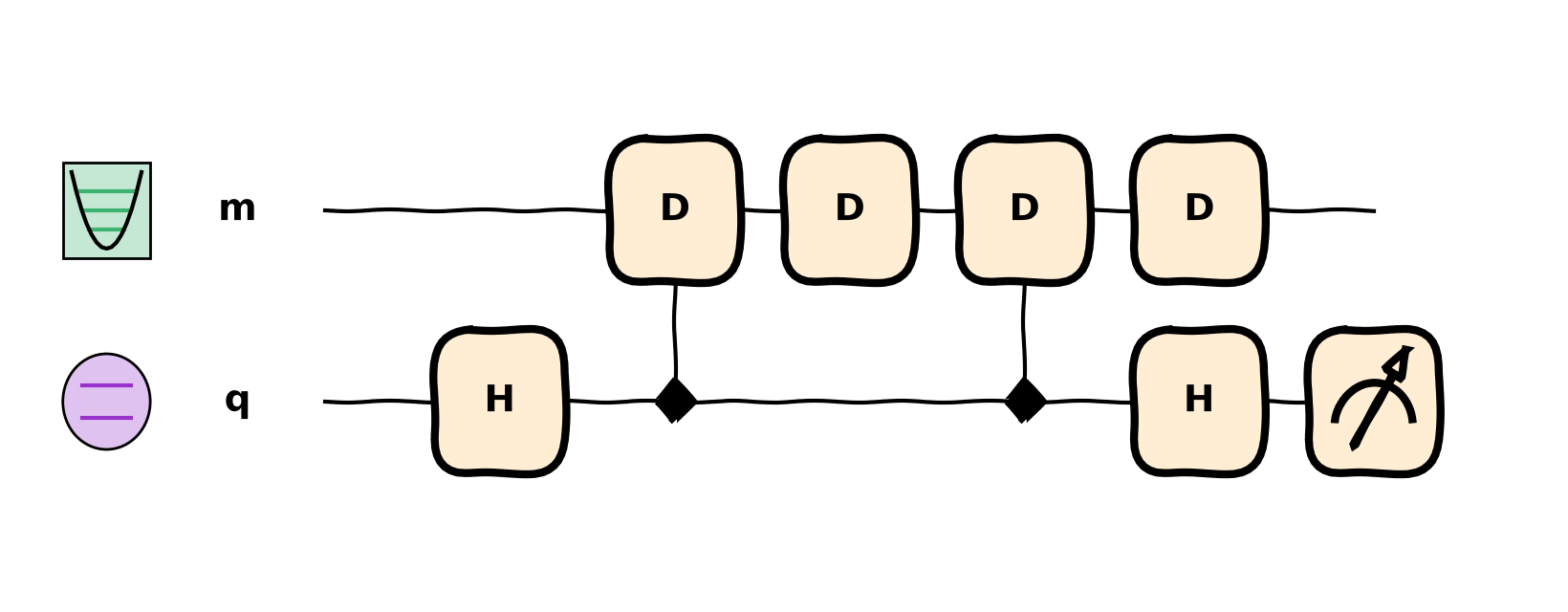
We’ll start by defining a quantum function for our circuit like usual, but we won’t bind it to a particular device. This circuit realizes a loop in phase space with area \(\beta^2\) whose orientation depends on the qubit state, and it effectively realizes an \(R_X(-4\beta^2)\) gate on the qubit.
import matplotlib.pyplot as plt
import numpy as np
import pennylane as qp

import hybridlane as hl

def cd_qfunc(beta):
    qp.H("q")
    hl.CD(beta, 0, wires=["q", "m"])
    hl.D(beta, np.pi / 2, wires="m")
    hl.CD(-beta, 0, wires=["q", "m"])
    hl.D(-beta, np.pi / 2, wires="m")
    qp.H("q")

    return hl.expval(qp.Z("q"))

def _():
    fig = plt.figure()
    hl.draw_mpl(cd_qfunc, style="sketch", fig=fig)(2.0)
    return fig

_()
Simulation
To check that the circuit definition is correct, we’ll simulate it using default.hybrid by binding the function into a QNode using a different syntax than the typical annotation. We can compare the output of the circuit against its analytical expected value, \(\langle Z\rangle = \cos(4\beta^2)\).
from hybridlane.devices import DefaultHybrid

# Bind the qfunc to `default.hybrid`
sim_qnode = qp.QNode(cd_qfunc, DefaultHybrid(fock_level=32))

# Test out different sampled values of beta
beta_sample = np.linspace(0, 2, 40)
expval = [sim_qnode(beta) for beta in beta_sample]

# Exact expression above
beta_exact = np.linspace(0, 2, 250)
expval_exact = np.cos(4 * beta_exact**2)

fig = plt.figure()
plt.plot(beta_exact, expval_exact, label=r"$\cos(4\beta^2)$")
plt.scatter(beta_sample, expval, label="Samples")
plt.xlabel(r"$\beta$")
plt.ylabel(r"$\langle Z\rangle$")
plt.legend()
fig
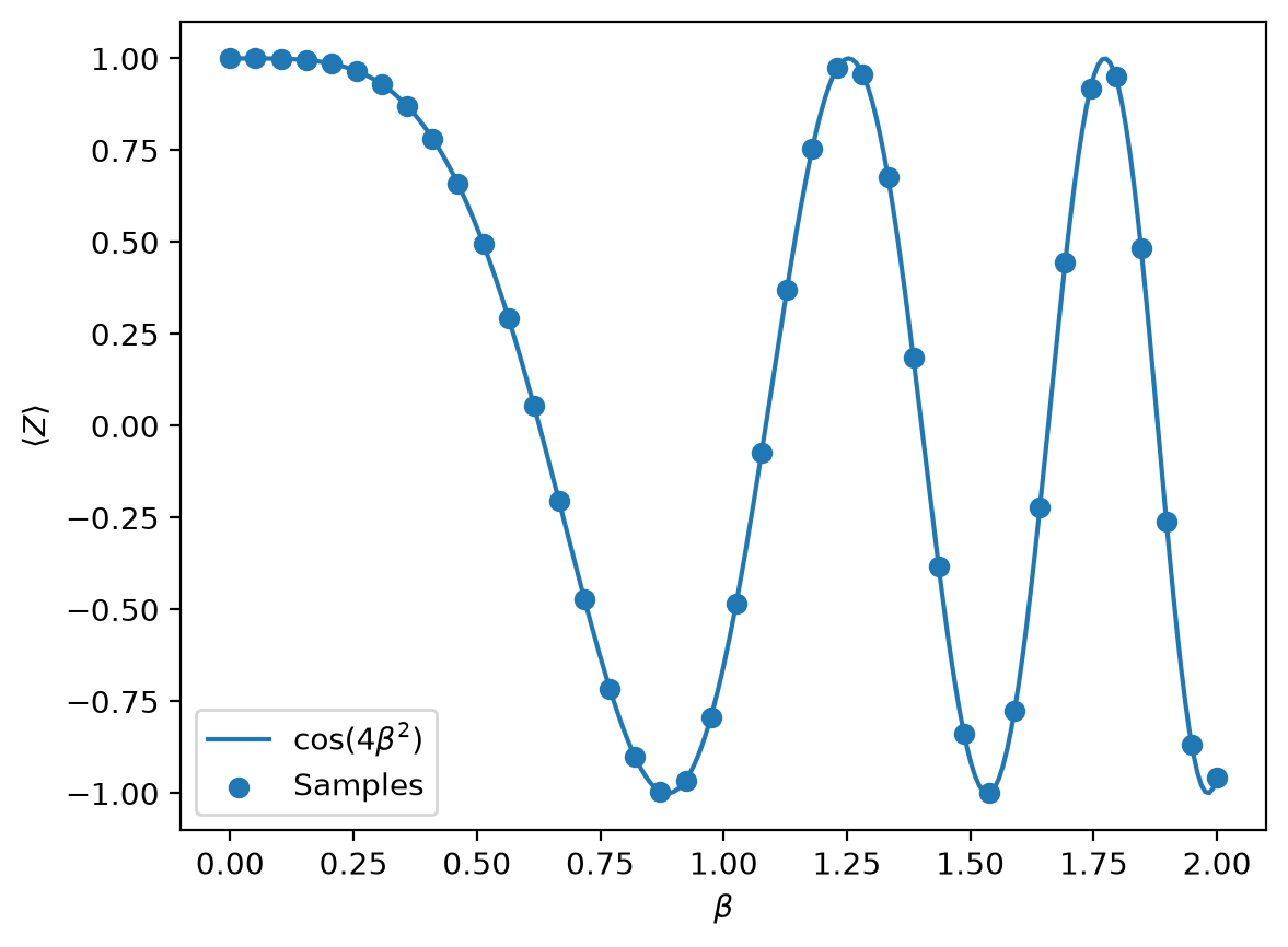
Our circuit matches the analytic result, so let’s move on to compiling it for hardware.
Cross-compiling
Now we’ll use the sandiaqscout.hybrid device, which implements a compilation target for a trapped-ion platform. Again, it’s worth mentioning that the workflow is the same for other devices and isn’t restricted to this particular backend.
In the same way as before, let’s bind the circuit definition to the hardware device.
from hybridlane.devices.sandia_qscout import QscoutIonTrap

# Bind to qscout device, also setting the shots because the ion trap doesn't
# work in "analytic" mode.
hw_qnode = qp.set_shots(qp.QNode(cd_qfunc, QscoutIonTrap(n_qubits=6)), 1024)
This device’s preprocessing transforms automatically take care of many transforms we’d have to do. We can use hl.draw_mpl to show the compiled circuit after it goes through all the preprocessing by using the level="device" parameter. Also, we’ll need the graph decomposition system.
qp.decomposition.enable_graph()

fig2 = plt.figure()
hl.draw_mpl(hw_qnode, level="device", style="sketch", fig=fig2)(2.0)
fig2
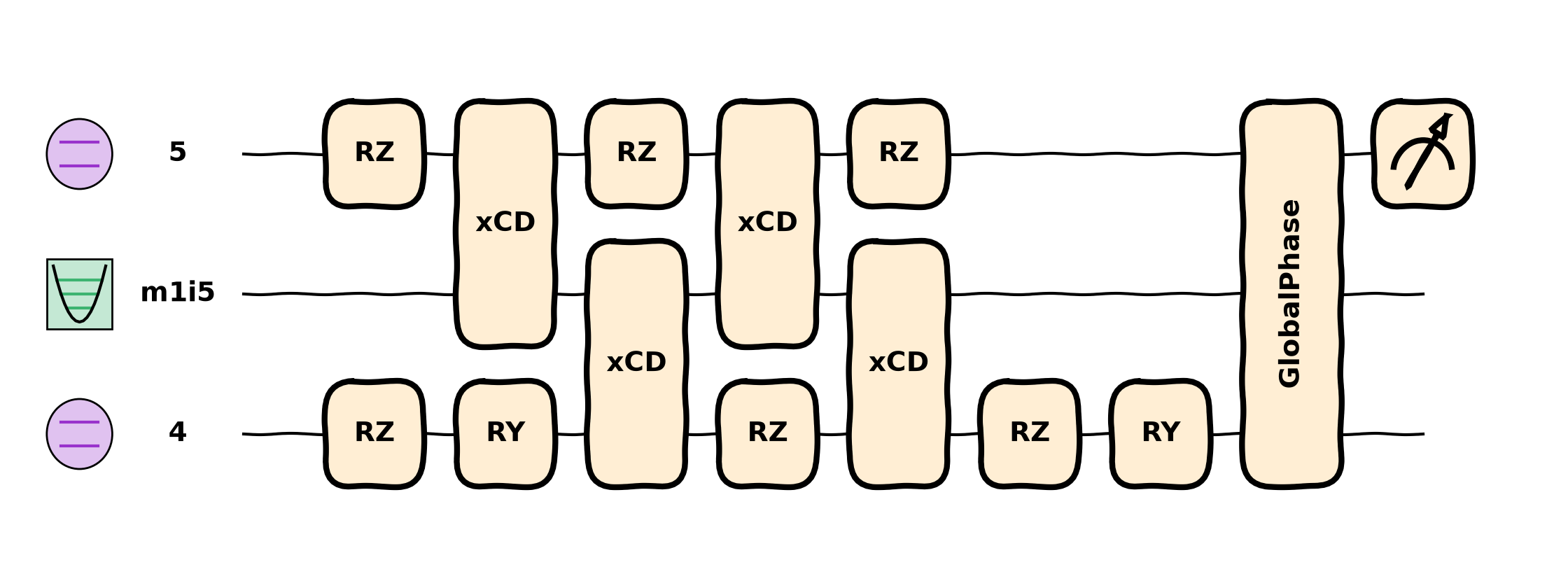
The compilation routine has performed many changes here
The \(D\) gates were realized through dynamic qubit allocation, and the resulting dynamic wires were converted back to normal wires with
resolve_dynamic_wires.The gates were converted to the native gates of the trap. For example, the 4 \(CD\) gates (after the above step) became \(xCD\) gates with some single-qubit rotations.
The algorithmic wire labels were mapped to hardware wire labels with a custom transform (e.g. mode
m -> m1i5).Adjacent qubit rotations were fused with
merge_rotations.
Alternatively, if you need the concrete QuantumScript after compilation, this can be obtained with qp.workflow.construct_tape:
tape = qp.workflow.construct_tape(hw_qnode, level="device")(2.0)
tape.operations
['RZ(np.float64(6.283185307179586), wires=[5])',
 'ConditionalXDisplacement(2.0, 0.0, wires=[5, Qumode(manifold=1, index=5)])',
 'RZ(np.float64(6.283185307179586), wires=[5])',
 'RZ(3.141592653589793, wires=[4])',
 'RY(1.5707963267948966, wires=[4])',
 'ConditionalXDisplacement(2.0, 1.5707963267948966, wires=[4, '
 'Qumode(manifold=1, index=5)])',
 'RZ(np.float64(6.283185307179586), wires=[4])',
 'ConditionalXDisplacement(-2.0, 0.0, wires=[5, Qumode(manifold=1, index=5)])',
 'RZ(np.float64(6.283185307179586), wires=[5])',
 'ConditionalXDisplacement(-2.0, 1.5707963267948966, wires=[4, '
 'Qumode(manifold=1, index=5)])',
 'RZ(3.141592653589793, wires=[4])',
 'RY(1.5707963267948966, wires=[4])',
 'GlobalPhase(-25.132741228718352, wires=[])']
While this notebook doesn’t actually run the resulting circuit on hardware, we’ve successfully replicated the workflow you find in mature qubit-based software. And if you’re working on quantum hardware or a simulator, building a Device will let you integrate your project into hybridlane so that you can program it at a high level.
OpenQASM
Suppose you need to serialize your circuit – maybe you’re building a device and have to send it over the network. hybridlane provides an intermediate representation (IR) based on OpenQASM 3.0 to facilitate this, with extensions to support CV-DV quantum programs.
As an example, we’ll serialize the above compiled circuit with hl.to_openqasm. The first step will be to teach hybridlane how to serialize the \(xCD\) gate because it’s not part of our standard library, which you can view here. The other gates are qubit gates that are part of the regular OpenQASM standard library.
To define a serializer for a gate, you register an implementation for format_gate_as_qasm. We’ll reuse the definition for \(CD\) and just change the op code:
from typing import Any

from hybridlane.io.openqasm import format_gate_as_qasm

@format_gate_as_qasm.register
def _(op: hl.XCD, wire_to_str: dict[Any, str], precision: int | None = None) -> str:
    if precision:
        params = [f"{p:.{precision}f}" for p in op.parameters]
    else:
        params = list(map(str, op.parameters))

    gate_name = "cv_xcd"
    wires = [wire_to_str[w] for w in op.wires]
    param_str = "(" + ", ".join(params) + ")" if params else ""
    wire_str = ", ".join(wires)
    gate_str = f"{gate_name}{param_str} {wire_str};"
    return gate_str
The arguments to the implementation are:
op: The operator that is being encoded.wire_to_str: A dictionary mapping the wires in the circuit to their OpenQASM labels (e.g.m -> m[3]).precision: An optional number of decimal places to use when writing out angle parameters.
Additionally, the implementation must follow the rules of functools.singledispatch in order for it to work properly, for which you have two options:
The primary format is to type-hint the variable
op: hl.XCD. You can reuse an implementation for multiple gates by using a union type likehl.XCD | hl.YCD.You could choose to pass the operator type to the decorator instead like
@format_gate_as_qasm.register(hl.XCD), particularly if you’re programmatically generating some implementations.
With this accomplised, let’s encode our circuit. hl.to_openqasm uses the familiar functional style you’ve seen in many PennyLane functions like qp.specs.
ir = hl.to_openqasm(hw_qnode, level="device", precision=5)(2.0)
print(ir)
OPENQASM 3.0;
include "stdgates.inc";
include "cvstdgates.inc";

qubit[2] q;
qumode[1] m;

def state_prep() {
    reset q;
    reset m;
    rz(6.28319) q[0];
    cv_xcd(2.00000, 0.00000) q[0], m[0];
    rz(6.28319) q[0];
    rz(3.14159) q[1];
    ry(1.57080) q[1];
    cv_xcd(2.00000, 1.57080) q[1], m[0];
    rz(6.28319) q[1];
    cv_xcd(-2.00000, 0.00000) q[0], m[0];
    rz(6.28319) q[0];
    cv_xcd(-2.00000, 1.57080) q[1], m[0];
    rz(3.14159) q[1];
    ry(1.57080) q[1];
    gphase(-25.13274) ;
}

state_prep();
bit[1] c0;
c0[0] = measure q[0];
Evident from the above example, hybridlane’s OpenQASM added a few modifications:
It includes both the OpenQASM standard library of qubit gates (
stdgates.inc) and our custom CV-DV standard library (cvstdgates.inc).The register definitions preserved the type information, with a dedicated qumode register
m.Our non-standard \(xCD\) gate was encoded as
cv_xcdin thestate_prep()routine.
Parsing this would require a modified OpenQASM parser, but that could be created relatively easily by adjusting the grammar definition.