First Program¶

import marimo as mo

Heterogeneous quantum computing¶

hybridlane implements hetereogeneous quantum programming, enabling you to define quantum circuits that incorporate both qubits and qumodes. To illustrate how this differs from normal quantum programs in PennyLane, we’ll consider a circuit made entirely of PennyLane gates:

import pennylane as qp

default_qubit = qp.device("default.qubit")

@qp.qnode(default_qubit)
def qubit_circuit1():
    qp.H(0)
    qp.CNOT((0, 1))
    return qp.state()

qubit_circuit1()

array([0.70710678+0.j, 0.        +0.j, 0.        +0.j, 0.70710678+0.j])

This of course produces the well-known Bell state \(\ket{\phi^+} = \frac{1}{\sqrt{2}}(\ket{00} + \ket{11})\). So far, it’s a well-formed PennyLane program.

Now let’s add a continuous-variable (CV) gate acting on a third wire, which won’t touch the first two. In principle, this is a perfectly valid quantum program.

@qp.qnode(default_qubit)
def qubit_circuit2():
    qp.H(0)
    qp.CNOT((0, 1))
    qp.Displacement(0.5, 0, wires=2)
    return qp.state()

try:
    qubit_circuit2()
except Exception as e:
    print(e)

Operator Displacement(0.5, 0, wires=[2]) not supported with default.qubit and does not provide a decomposition.

We get an error that the displacement gate is not supported on default.qubit (granted, the device name tells you that it specializes to qubit gates). You would see a similar thing if you tried adding qubit gates to a circuit bound to default.gaussian – and indeed, no PennyLane device lets you mix qubit and qumode gates in the same circuit.

This is where hybridlane comes in. We can run the exact same circuit that just errored on hybridlane’s default.hybrid device.

import hybridlane as hl

default_hybrid = qp.device("default.hybrid", fock_level=8)

@qp.qnode(default_hybrid)
def circuit1():
    qp.H(0)
    qp.CNOT((0, 1))
    qp.Displacement(0.5, 0, wires=2)
    return hl.state()  # note we did have to replace qp.state -> hl.state

state = circuit1()
state.shape

[32]

The state has the dimension we expect for the composite Hilbert space \(dim(\mathbb{C}^2 \otimes \mathbb{C}^2 \otimes \mathbb{C}^{8}) = 32\). But this circuit doesn’t really do anything interesting – because its gates don’t induce interactions between the qubits (0,1) and the qumode 2, you could have simulated this by splitting the circuit and dispatching each part to the appropriate PennyLane device.

A hybrid circuit¶

Let’s now build a hybrid circuit that has qubit-qumode interactions. We’ll recycle the Bell state example, but instead of entangling 2 qubits, we can entangle a qubit and a qumode. This example prepares the state \(\frac{1}{\mathcal{N}}(\ket{0,\alpha} + \ket{1,-\alpha})\), where \(\ket{\alpha}\) is the CV coherent state and \(\mathcal{N}\) is a normalization factor resulting from the fact that two coherent states are not perfectly orthogonal.

@qp.qnode(default_hybrid)
def circuit2(alpha):
    qp.H(0)
    hl.CD(alpha, 0, wires=(0, 1))
    return hl.state()

Here we use the conditional displacement (CD) gate \(CD(\alpha) = \exp[Z\otimes(\alpha a^\dagger - \alpha^* a)]\), which is similar to a qubit-controlled operation in PennyLane, except that it has the form

\[CD(\alpha) = \ket{0}\bra{0} \otimes D(\alpha) + \ket{1}\bra{1} \otimes D(-\alpha),\]

applying a unitary if the qubit is in state \(\ket{0}\) and its inverse otherwise. We can inspect the state of the qumode based on the qubit and see that we got the correct expression:

state2 = circuit2(1.0).reshape(2, -1)
print(f"Qubit |0>: {state2[0]}")
print(f"Qubit |1>: {state2[1]}")

Qubit |0>: [0.42888194+0.j 0.42888196+0.j 0.30326516+0.j 0.17509166+0.j
 0.08753677+0.j 0.03919483+0.j 0.0157952 +0.j 0.00672991+0.j]
Qubit |1>: [ 0.42888194+0.j -0.42888196+0.j  0.30326516+0.j -0.17509166+0.j
  0.08753677+0.j -0.03919483+0.j  0.0157952 +0.j -0.00672991+0.j]

Type checking¶

hybridlane is able to handle the heterogeneous circuits above through type inference. It inspects the circuit operations to determine which wires are qubits and which are qumodes, and to enforce consistency. We won’t go into much detail here, but one way to see what the type checker has deduced is by drawing the circuit with hl.draw_mpl, which returns a function accepting the parameters of your circuit that then produces the plot.

This is very much like PennyLane’s draw_mpl, but we also show the wire type icons determined by the type checker.

import matplotlib.pyplot as plt

fig = plt.figure()
hl.draw_mpl(circuit2, style="sketch", fig=fig)(1.0)
fig

png

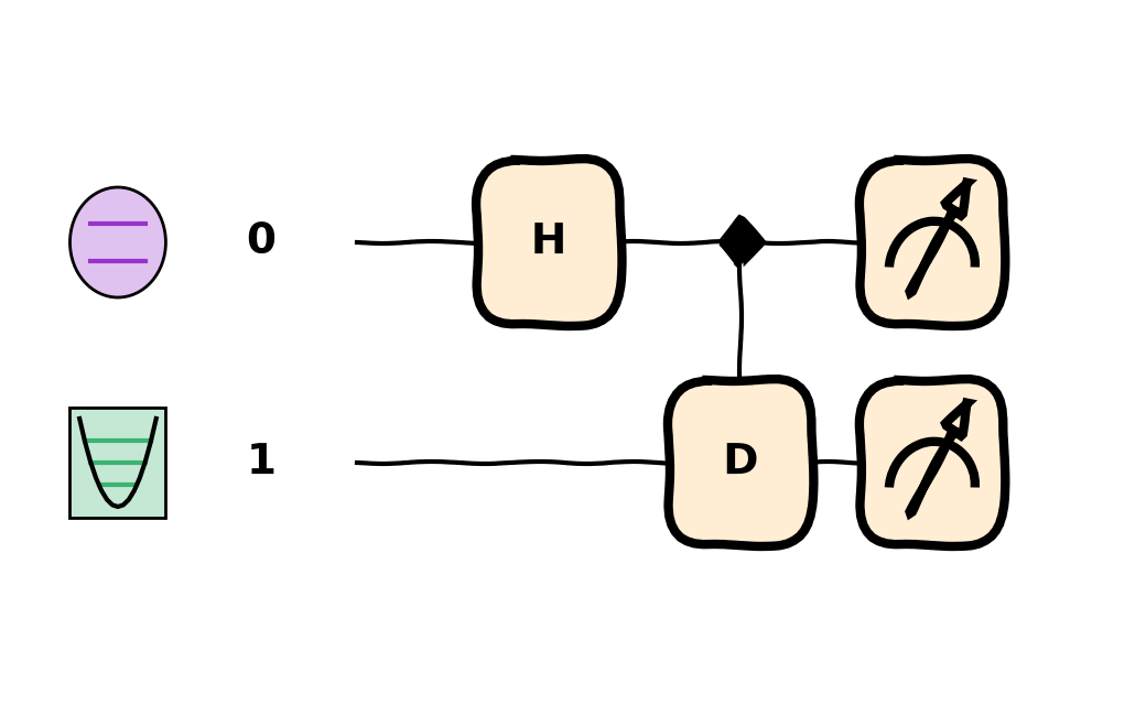
You can also perform this check programmatically by manually invoking hybridlane’s type checker:

result = hl.type_check(circuit2)(1.0)
result.wire_types

OrderedDict({0: Qubit(), 1: Qumode()})

Now that you’ve seen how to define a hybrid circuit, you can see a full list of the available CV and hybrid gates available at the documentation. Don’t forget you can use the qubit gates from PennyLane too!

When to use `hl` vs. `qp`¶

It may get confusing at first navigating when to call PennyLane (qp) versus hybridlane (hl). After all, you can use PennyLane gates, and there are some shared gates between the libraries. Here’s some simple rules that will get you 95% of the way there:

Choose qp if you’re

using a qubit gate or algorithm (e.g. qp.X, qp.RZ)
counting gates with qp.specs
creating a device with qp.device or binding a function using qp.qnode

Choose hl if you’re

using CV or hybrid gates and algorithms (e.g. hl.D, hl.JC)
performing measurements at the end of a quantum function (e.g. hl.expval)
drawing a circuit with matplotlib (hl.draw_mpl)
doing math with hl.math

And in general, prefer using hl; we only override functions as necessary.

First Program¶

Heterogeneous quantum computing¶

A hybrid circuit¶

Type checking¶

When to use hl vs. qp¶

When to use `hl` vs. `qp`¶