Gate Decompositions
import marimo as mo
Symbolic op math
In this notebook, we’ll demonstrate how to perform some symbolic gate decomposition in hybridlane. We heavily leverage PennyLane’s graph decomposition system, so you’ll need to enable that
import matplotlib.pyplot as plt
import numpy as np
import pennylane as qp

import hybridlane as hl

qp.decomposition.enable_graph()
Here are the primary symbolic functions that you can use:
qp.adjoint: Takes the adjoint of an operator \(U \mapsto U^\dagger\)
qp.pow: Takes powers of an operator, \(U \mapsto U^z\)
qp.ctrl: Controls a unitary on the state of one or more qubits, e.g. \(U \mapsto \Pi_0 I + \Pi_1 U\)
hl.qcond: Conditions a unitary on the state of a qubit. \(U \mapsto \Pi_0 U + \Pi_1 U^\dagger\)
Note that while hl.qcond realizes a similar thing to qp.ctrl, it’s such a common pattern in CV-DV computing that hybridlane adds it as a distinct symbolic operation.
qp.adjoint
PennyLane’s qp.adjoint function allows taking the inverse of a single gate or an entire quantum function, and hybridlane’s gates are programmed to interoperate with it. The canonical way to use it is with its functional form. For an operator op taking arguments *args, the adjoint can be performed like qp.adjoint(op) -> f(*args) – that is, qp.adjoint takes an operator or quantum function and returns a new function accepting the arguments of the original operator or quantum function.
Here’s an example of a single \(CR\) gate being inverted:
inv_cr = qp.adjoint(hl.CR)
inv_cr(0.123, wires=(0, 1))
Adjoint(ConditionalRotation(0.123, wires=[0, 1]))
Often, this will be inlined like
qp.adjoint(hl.CR)(0.123, wires=(0, 1))
Adjoint(ConditionalRotation(0.123, wires=[0, 1]))
The qp.adjoint function is lazy by default, so it simply wraps our operator in the Adjoint type. This is usually a good thing as it works best with PennyLane’s graph decomposition system, but if you’d like it to perform the operation eagerly, then we can pass lazy=False
qp.adjoint(hl.CR, lazy=False)(0.123, wires=(0, 1))
ConditionalRotation(-0.123, wires=[0, 1])
As you can see, it turned \(CR(\theta) \mapsto CR(-\theta)\). This saves you from having to program the adjoint yourself in your circuits. The argument to qp.adjoint can also be a quantum function calling several operations, so here’s an example of a circuit realizing the identity gate
dev = qp.device("default.hybrid", fock_level=16)

def custom_op(a):
    qp.H(0)
    hl.CD(a, 0, wires=(0, 1))

@qp.qnode(dev)
def circuit(a):
    custom_op(a)
    qp.adjoint(custom_op)(a)

    return hl.expval(hl.N(1))

def _():
    fig = plt.figure()
    hl.draw_mpl(circuit, level="device", style="sketch", fig=fig)(2.0)
    return fig

_()
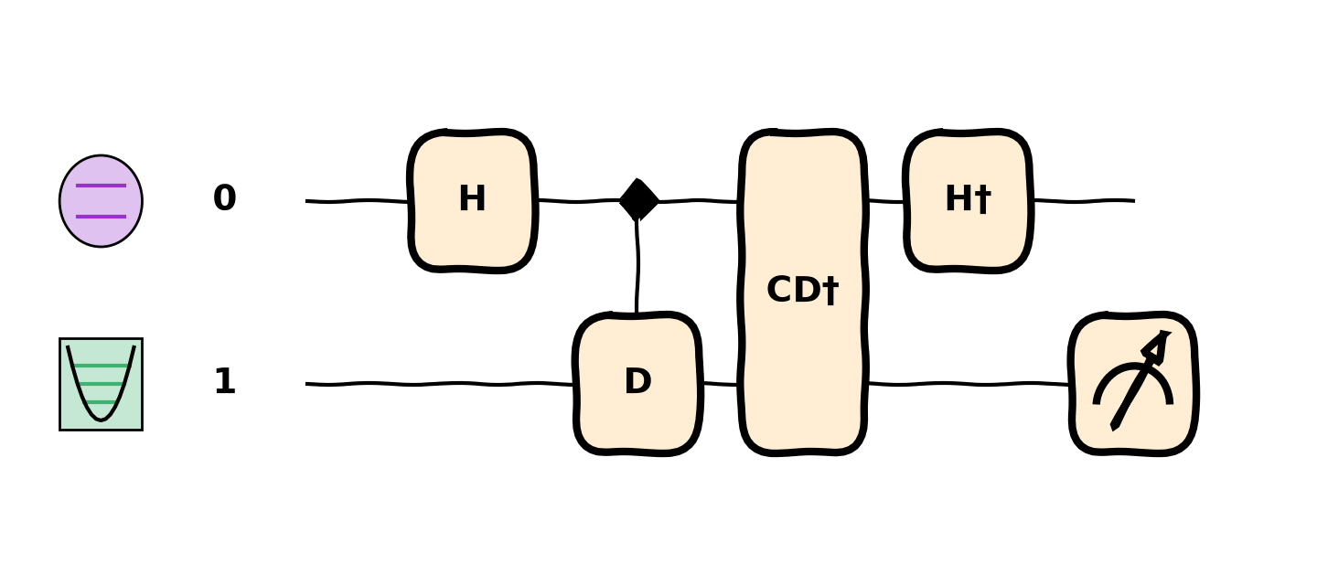
The qp.adjoint wrapper took care of reversing the operations and negating each, saving us some work.
qp.pow
qp.pow(op) raises an operator to a power. Here’s an example:
qp.pow(hl.JC(0.5, 0.123, wires=(0, 1)), z=2)
JaynesCummings(0.5, 0.123, wires=[0, 1])**2
It can also be accessed with **:
hl.JC(0.5, 0.123, wires=(0, 1)) ** 2
JaynesCummings(0.5, 0.123, wires=[0, 1])**2
And finally, both of those are lazy, so if want to eagerly evaluate it, then pass lazy=False
qp.pow(hl.JC(0.5, 0.123, wires=(0, 1)), z=2, lazy=False)
JaynesCummings(1.0, 0.123, wires=[0, 1])
qp.ctrl
This has similar usage to qp.adjoint. Here’s an example of realizing a displacement that’s not symmetric about the origin, \(D_c(\alpha) = \Pi_0 I + \Pi_1 D(\alpha)\)
@qp.qnode(dev)
def circuit2(a):
    qp.H(1)
    qp.ctrl(hl.D, control=[1])(a, 0, wires=0)
    return hl.expval(hl.X(0))

def _():
    fig = plt.figure()
    hl.draw_mpl(circuit2, level="device", style="sketch", fig=fig)(2.0)
    return fig

_()
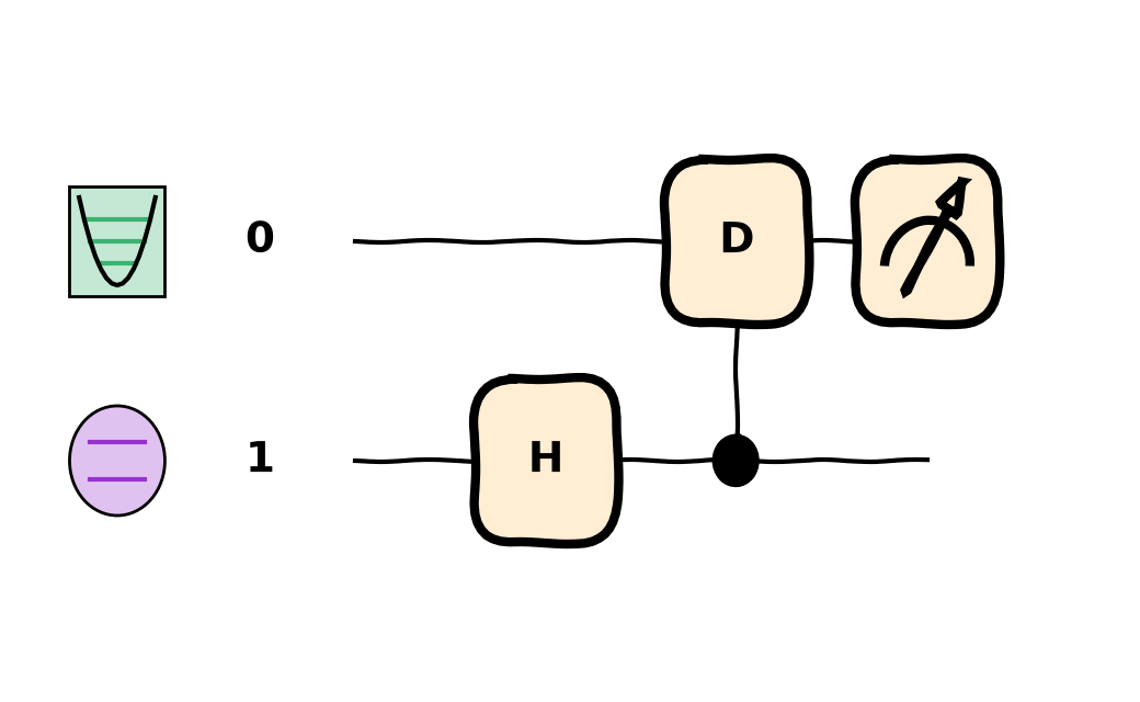
If we evaluate it, we’ll see we get a nonzero value of \(\langle \hat{x} \rangle\), whereas we would obtain 0 with a symmetric conditional displacement \(CD\).
circuit2(2.0)
array(1.414192)
hybridlane has some symbolic rules that enable it to decompose that gate in terms of the more native \(CD\) gate
decomposed = qp.decompose(circuit2, gate_set={qp.H, hl.D, hl.CD})
decomposed_tape = qp.workflow.construct_tape(decomposed)(2.0)
decomposed_tape.operations
['H(1)',
 'Displacement(1.0, 0, wires=[0])',
 'ConditionalDisplacement(1.0, 3.141592653589793, wires=[1, 0])']
hl.qcond
This is a special symbolic operation unique to hybridlane. If you express your unitary as \(U = e^{-i \theta G}\), then this symbolic operation performs \(U \mapsto e^{-i \theta Z \otimes G}\), where \(Z\) is the Pauli \(Z\) on the conditioning qubit. This symbolic identity comes up often in hybrid CV-DV computing: qcond(D) -> CD, qcond(BS) -> CBS, and so on. For example,
hl.qcond(hl.D(0.123, 0, wires=0), control_wires=[1])
ConditionalDisplacement(0.123, 0, wires=[1, 0])
You can also use it to condition a gate on multiple qubits, like \(U = e^{-i \theta Z \otimes Z \otimes G}\), and hybridlane can decompose that using CNOT gates if required
@qp.decompose(gate_set={qp.CNOT, hl.CBS})
@qp.qnode(dev)
def qcond_circuit():
    hl.qcond(hl.BS, control_wires=[2, 3])(0.123, 0, wires=(0, 1))
    return hl.state()

def _():
    fig = plt.figure()
    hl.draw_mpl(qcond_circuit, style="sketch", fig=fig)()
    return fig

_()
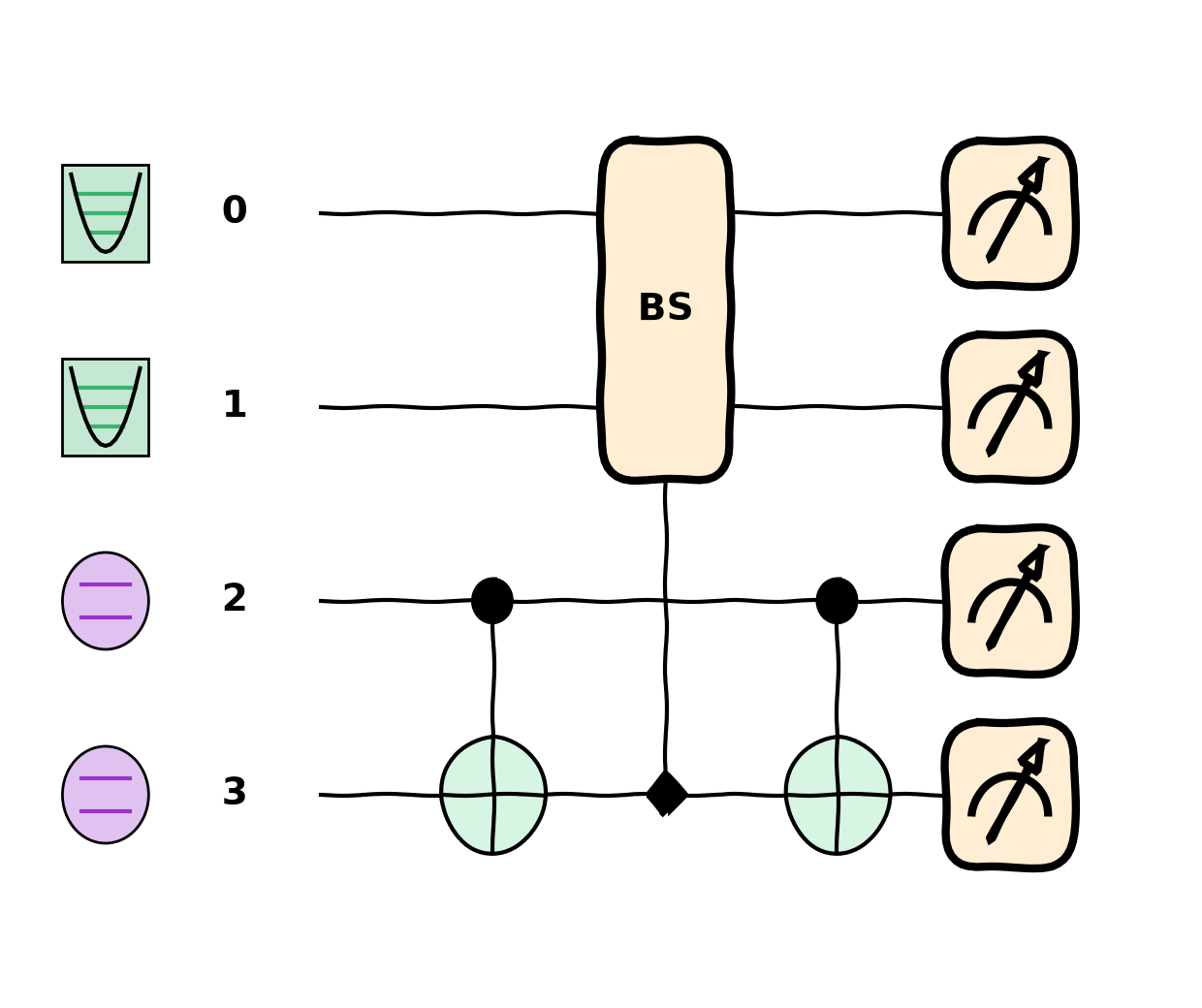
Gate decompositions
Symbolic op math is really important in the decomposition system. Now we’ll talk about how to invoke the decomposition system. In addition to some of the decompositions you’ve seen above, hybridlane has many more from Liu et al and Crane et al.
You can invoke the decomposition system using the PennyLane transform qp.decompose, which to first order, accepts your desired gate set. Here’s one decomposition for the \(CBS\) gate from Crane et al, targetted to superconducting hardware:
@qp.decompose(gate_set={hl.BS, hl.CR})
@qp.qnode(dev)
def cbs_circuit():
    hl.CBS(2.0, 0, wires=(0, 1, 2))
    return hl.state()

def _():
    fig = plt.figure()
    hl.draw_mpl(cbs_circuit, style="sketch", fig=fig)()
    return fig

_()
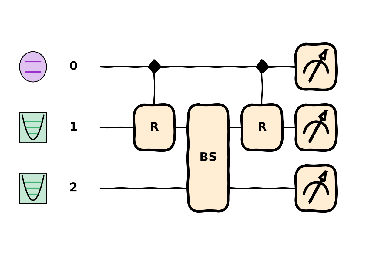
You can list all available decompositions for a gate using qp.list_decomps
qp.list_decomps(hl.CD)
DecompCollection([
    DecompositionRule(name=_cd_parity_decomp),
    DecompositionRule(name=_cd_to_ecd),
    DecompositionRule(name=_cd_to_xcd),
    DecompositionRule(name=_cd_to_rb)
])
Sometimes, depending on your target gate set, multiple rules can apply. qp.decompose lets you weight different target gates and it tries to pick the decomposition with the lowest total cost.
Gates can also be decomposed using dynamic qubit allocation (sorry, we haven’t yet implemented qumode allocation). As an example. some platforms like trapped-ion systems don’t natively support the \(D\) gate, but they do support a variant of the \(CD\) gate, the \(XCD\) gate, which displaces w.r.t. a different qubit axis. Thus, if we could find a clean, unused qubit in the state \(\ket{0}\), we could then realize a \(D\) gate with an \(XCD\) gate and some single-qubit gates.
You can instruct the decomposition system to use dynamic qubit allocation with the num_work_wires argument.
from hybridlane.ops.op_math.decompositions.qubit_conditioned_decompositions import (
    make_gate_with_ancilla_qubit,
)

# This also shows how to temporarily use some additional decomposition rules. here,
# make_gate_with_ancilla_qubit is a symbolic rule we made to use hl.qcond() under the hood.
@qp.decompose(
    gate_set={hl.XCD, qp.H},
    fixed_decomps={hl.D: make_gate_with_ancilla_qubit(hl.D)},
    num_work_wires=None,  # `None` allows as many qubits allocated as necessary
)
@qp.qnode(dev)
def dynamic_d_circuit():
    hl.D(2.0, 0, wires=0)
    return hl.state()

def _():
    tape = qp.workflow.construct_tape(dynamic_d_circuit)()
    return tape.operations

_()
['Allocate(wires=[<DynamicWire>])',
 'H(<DynamicWire>)',
 'ConditionalXDisplacement(2.0, 0, wires=[<DynamicWire>, 0])',
 'H(<DynamicWire>)',
 'Deallocate(wires=[<DynamicWire>])']
You can find more information on how to work with their graph decomposition system here.
Quantum phase estimation
Putting all this together, let’s see how these decomposition identities can be used to synthesize a high-level algorithmic primitive: the quantum phase estimation. We can use it to perform a Fock state readout using qubits (albeit an expensive one). The hamiltonian of our system will be \(H = \hat{n}\), whose time evolution is the familiar phase-space rotation \(R(\theta) = e^{-i\theta\hat{n}}\).
from pprint import pprint

from hybridlane.wires import BasisMap, ComputationalBasis

# We have to build the unitary outside the circuit so it isn't queued
# into the circuit's operations
op = hl.R(1.0, wires="m")

@qp.decompose(
    gate_set={hl.R, hl.CR, qp.CNOT, qp.H, qp.ControlledPhaseShift, qp.SWAP, qp.FockState}
)
@qp.set_shots(10)
@qp.qnode(dev)
def qpe(n, n_bits):
    # This is just for illustration, you could prepare any state prior
    qp.FockState(n, wires="m")

    wires = range(n_bits)
    qp.QuantumPhaseEstimation(op, estimation_wires=wires)

    # Sample computational bitstrings
    map = BasisMap({wires: ComputationalBasis.Discrete})
    return hl.sample(schema=map)

bitstrings = qpe(4, n_bits=4)
pprint(bitstrings)
SampleResult(data={0: array([0, 0, 0, 0, 0, 0, 0, 0, 0, 0]),
                   1: array([1, 1, 1, 1, 1, 1, 1, 1, 1, 0]),
                   2: array([1, 1, 1, 1, 1, 1, 1, 1, 1, 1]),
                   3: array([0, 0, 0, 0, 0, 0, 0, 0, 0, 0])},
             bases=BasisMap({[0, 1, 2, 3]: ComputationalBasis.Discrete}))
Behind the scenes, many identities have been chained together to realize the controlled unitary \(C(R(\theta) ^ k)\). We can also illustrate here how to do some resource estimation with qp.specs.
for n_bits in (2, 4, 8, 16):
    specs = qp.specs(qpe)(4, n_bits)
    print(f"{n_bits} bits")
    print("==============")
    print(specs)
    print()
2 bits
==============
Device: default.hybrid
Device wires: None
Shots: Shots(total=10)
Level: gradient

Wire allocations: 3
Total gates: 11
Gate counts:
- FockState: 1
- Hadamard: 4
- Rotation: 2
- ConditionalRotation: 2
- SWAP: 1
- ControlledPhaseShift: 1
Measurements:
- sample(2 wires): 1
Depth: 9

4 bits
==============
Device: default.hybrid
Device wires: None
Shots: Shots(total=10)
Level: gradient

Wire allocations: 5
Total gates: 25
Gate counts:
- FockState: 1
- Hadamard: 8
- Rotation: 4
- ConditionalRotation: 4
- SWAP: 2
- ControlledPhaseShift: 6
Measurements:
- sample(4 wires): 1
Depth: 17

8 bits
==============
Device: default.hybrid
Device wires: None
Shots: Shots(total=10)
Level: gradient

Wire allocations: 9
Total gates: 65
Gate counts:
- FockState: 1
- Hadamard: 16
- Rotation: 8
- ConditionalRotation: 8
- SWAP: 4
- ControlledPhaseShift: 28
Measurements:
- sample(8 wires): 1
Depth: 33

16 bits
==============
Device: default.hybrid
Device wires: None
Shots: Shots(total=10)
Level: gradient

Wire allocations: 17
Total gates: 193
Gate counts:
- FockState: 1
- Hadamard: 32
- Rotation: 16
- ConditionalRotation: 16
- SWAP: 8
- ControlledPhaseShift: 120
Measurements:
- sample(16 wires): 1
Depth: 65