Package installation

You can install the package from CRAN or from GitHub:

install.packages("Smisc")

# If devtools is not already installed, do this:
install.packages("devtools") 

# Now install the package
devtools::install_github("pnnl/Smisc")

library(Smisc)

Load objects to a name of choice

I always found it a bit annoying how load() places the object(s) in the .Rdata file into .GlobalEnv without immediately telling you what the name(s) of the object is (are). loadObject() makes it easy to assign the contents of the .Rdata file to an object of my choice, like this:

myName <- loadObject("~/aDir/aFile.Rdata")

And thus myName contains the contents aFile.Rdata.

Flexibly ingest data

dataIn() provides a flexible way to ingest data into R. It takes a single argument that can be the filename of an .Rdata or .csv file, a package dataset, or an existing data frame. It returns a data frame. Each of these, in principle, would achieve the same result, regardless of the format of the input data:

# Read a csv file
d <- dataIn("someData.csv")

# Load a .Rdata file
d <- dataIn("someData.Rdata")

# If the dataframe already exists as "someData"
d <- dataIn(someData)

# If "someData" is in the package "somePackage"
d <- dataIn("somePackage::someData")

Identify missing columns or rows

Sometimes it’s handy to know whether all the elements in a given row (or column) of a matrix or data frame are missing. allMissing() returns a logical vector indicating whether all the elements in a row (or column) are missing. It’s a nice compliment to complete.cases().

# A dataframe with a missing column
m <- data.frame(A = rnorm(3), B = NA, C = letters[3])
m

           A  B C
1 -1.2070657 NA c
2  0.2774292 NA c
3  1.0844412 NA c

allMissing(m, byRow = FALSE)

    A     B     C 
FALSE  TRUE FALSE 

Compare two data frames

dframeEquiv() compares two data frames (or two matrices) and determines whether they are equivalent or how they differ.

# Create two slightly different data frames
d1 <- data.frame(A = 1:2, B = c("a", "b"))
d2 <- data.frame(A = 1:2, B = c("a", "c"))

# Compare the dataframes
compare <- dframeEquiv(d1, d2)

75% of the elements of 'd1' and 'd2' are equivalent.

We can see the locations by index where the dataframes differ:

compare$loc.inequiv

  row.loc col.loc
1       2       2

And we can see a logical matrix indicating where they differ:

compare$equiv.matrix

     [,1]  [,2]
[1,] TRUE  TRUE
[2,] TRUE FALSE

Rapidly combine or bind numerous objects

Have you ever needed to row bind, rbind(), or column bind, cbind(), or combine/concatenate, c(), numerous objects, usually of the same type? If you do it iteratively, you’ll slow your machine to a crawl:

# The names of the 100 matrices, m1, m2, ..., m100
mNames <- paste("m", 1:100, sep = "")

# Initialize the combined object
combined <- NULL

# Now wait forever
for (m in mNames) {
  combined <- rbind(combined, get(m))
}

qbind() provides a syntactically simple and fast solution:

# The names of the 100 matrices, m1, m2, ..., m100
mNames <- paste("m", 1:100)

# Now combined using `rbind()`
combined <- qbind(mNames, type = "row")

Row bind heterogenous matrices

Have you ever needed to row bind multiple matrices together that didn’t all have the same column names? smartRbindMat() function rapidly row binds them together by creating a final matrix with the union of the columns of the source matrices.

x <- as.matrix(data.frame(a = 1:2, b = 3:4))
y <- as.matrix(data.frame(a = 1:2, c = 5:6))
z <- as.matrix(data.frame(b = 7:8, d = 9:10))
smartRbindMat(x, y, z)

      a  b  c  d
[1,]  1  3 NA NA
[2,]  2  4 NA NA
[3,]  1 NA  5 NA
[4,]  2 NA  6 NA
[5,] NA  7 NA  9
[6,] NA  8 NA 10

Consistently select rows or columns

Have you ever selected a single row or column from a dataframe or matrix only to have R return an object structured in a way you weren’t expecting? select() makes R’s behavior consistent, always returning a matrix or dataframe with a single row or column, if necessary. It is especially useful in the situation where the number of rows or columns to be selected is variable and not necessarily known before hand.

# A simple dataframe
x <- data.frame(a = 1:2, b = 3:4)

# If we select a single column the usual way, we get a vector:
x[,1]

[1] 1 2

# But if we use select(), we get a single column dataframe
select(x, 1)

  a
1 1
2 2

Row-wise conversion of a dataframe to a list

df2list() converts a dataframe to a list, in a row-wise fashion (as opposed to as.list(), which converts in a column-wise fashion):

d <- data.frame(a = 1:2, b = letters[1:2])
d

  a b
1 1 a
2 2 b

df2list(d)

$`1`
$`1`$a
[1] 1

$`1`$b
[1] "a"


$`2`
$`2`$a
[1] 2

$`2`$b
[1] "b"

Convert a list to a dataframe

I use list2df() probably more than any other Smisc function. It converts a list of suitable object types (vectors, dataframes, or lists) into a single dataframe. It’s especially useful for collecting the output from strsplit(), or the results from lapply().

z <- list(a = c(first = 10, second = 12), b = c(first = 15, second = 17))
z

$a
 first second 
    10     12 

$b
 first second 
    15     17 

list2df(z)

  first second
a    10     12
b    15     17

Separate a list into separate objects

On occasion, it is useful to break a list into its separate elements and not have to refer to them using the list name. sepList() makes it easy:

# A simple list that we'll separate
aList <- list(x1 = 10, x2 = "a") 
sepList(aList)

# 'x1' is now in the Global environment:
x1

[1] 10

# And so is 'x2'
x2

[1] "a"

Convert factors to character variables in a dataframe

When creating a dataframe, the default behavior of R is to render all character variables as factors—which you may not want. factor2character() will convert all the factor variables in a dataframe to character.

myData <- data.frame(x = 10, y = "a", z = "b")
str(myData)

'data.frame':   1 obs. of  3 variables:
 $ x: num 10
 $ y: chr "a"
 $ z: chr "b"

myData1 <- factor2character(myData)
str(myData1)

'data.frame':   1 obs. of  3 variables:
 $ x: num 10
 $ y: chr "a"
 $ z: chr "b"

Convert factor to numeric

Naively attempting to convert a factor to a numeric vector can easily go wrong. For example, as.numeric() probably won’t give you what you’re looking for. factor2numeric() correctly converts a factor to a numeric vector.

x <- factor(c(4, 7))
x

[1] 4 7
Levels: 4 7

# Wrong
as.numeric(x)

[1] 1 2

# Right
factor2numeric(x)

[1] 4 7

Convert to numeric, if possible

as.numericSilent() is used by list2df() to create numeric variables if possible in the resulting dataframe. It can also be used to attempt the conversion of any vector to a numeric vector. If any warnings or errors are produced in the attempt, conversion to numeric does not take place, and the original vector is returned.

# A character vector of numbers
x <- c("1", "2", "3")

# Conversion takes place
as.numericSilent(x)

[1] 1 2 3

# A character vector of letters
y <- c("a", "b", "c")

# Conversion is not possible, so the original character vector is returned 
# with no complaints
as.numericSilent(y)

[1] "a" "b" "c"

Get a filename extension

getExtension() grabs the characters that make up the extensions of a vector of filenames.

getExtension(c("~/aDir/aFile.txt", "anotherFile.R"))

[1] "txt" "R"  

Get the path of a filename

getPath() grabs the characters that make up the pathname of a vector of filenames.

getPath(c("~/aDir/aFile.txt", "anotherFile.R"))

[1] "~/aDir" "."     

Strip a the extension from a filename

stripExtension() removes the characters that make up the extensions of a vector of filenames.

stripExtension(c("~/aDir/aFile.txt", "anotherFile.R"))

[1] "~/aDir/aFile" "anotherFile" 

Strip the path from a filename

stripPath() removes the characters that make up the pathname of a vector of filenames.

stripPath(c("~/aDir/aFile.txt", "anotherFile.R"))

[1] "aFile.txt"     "anotherFile.R"

Get the last set of characters after a delimiter

grabLast() is a more general function that is very similar to getExtension(): it selects the final set of characters that appear after a single-character delimiter. It is used by getExtension() and stripPath().

grabLast("some_new_stuff", "_")

[1] "stuff"

Embed a timestamp in a filename

timeStamp() embeds a the current date and time into the name of a file.

timeStamp("thisFile", "txt")

[1] "thisFile_2020-10-14_115309.txt"

Pad a numeric value with zeros

padZero() pads a numeric vector with zeros so that each element in the vector either has the same number of characters or the same number of trailing decimal places. This can be helpful in managing multiple files where files are sorted alpha-numerically.

# These files will sort in numeric order with the padded zeros
paste("fileNumber_", padZero(c(1, 10, 100)), ".txt", sep = "")

[1] "fileNumber_001.txt" "fileNumber_010.txt" "fileNumber_100.txt"

# An example of adding 0's to the right side
padZero(c(1.2, 1.34, 1.399), side = "r")

[1] "1.200" "1.340" "1.399"

Generate a hard-coded vector

When writing a script for analysis, have you ever wanted to select a bunch of columns (by name) in a dataframe, and had to extensively edit the output of colnames(myData) in order to have some tidy code in your script? hardCode() makes it easy to do this:

myData <- data.frame(a = 1:4, 
                     b = letters[1:4], 
                     c = rep(c(TRUE, FALSE), each = 2), 
                     d = rnorm(4))

hardCode(colnames(myData)[-1], vname = "myNewCols", vert = FALSE)

Pay close attention: what you see below is the output from the call to hardCode() that appears in the R console:

myNewCols <- c("b", "c", "d")   

Then you can copy and paste the code snippet above into your script and use it to select a subset of the data:

myNewCols <- c("b", "c", "d")
myData[,myNewCols]

  b     c          d
1 a  TRUE -2.3456977
2 b  TRUE  0.4291247
3 c FALSE  0.5060559
4 d FALSE -0.5747400

Granted, this is a trivial example, but when you have dozens of columns, this can make life a little easier. hardCode() can be used for more than just selecting column names: it can be used to hard code any type of vector that you might want to copy into a script.

Display the contents of a text file

more() prints the contents of a text file (stored on disk) in the R console, just like the more command in Unix—making it easy to see what’s in a file without having to leave the R console.

# Write a simple text file
cat("Here's a simple\n", "text file\n", 
    file = "simpleFile.txt", sep = "")

# Display using more()
more("simpleFile.txt")

Here's a simple
text file 

Print the object name and its value

pvar() stands for print variable, which makes it easy to see both the name and the value of an R object. pvar() is particularly useful for displaying the value of objects that are atomic (i.e. of length 1).

x <- "gratican"
y <- 3.14
pvar(x, y)

x = gratican; y = 3.14 

I often use it to troubleshoot loops, where I’d like to see the value of variables as the code progresses through the loop:

for (i in 1:2) {
  for (j in c("a", "b")) {
    pvar(i, j)
  }
}

i = 1; j = a 
i = 1; j = b 
i = 2; j = a 
i = 2; j = b 

Flexibly select valid elements from a character vector

I often write functions where one or more of the arguments are a vector of column names (or numbers) that will be selected from a dataframe. selectElements() provides a mechanism for selecting the columns using three different methods (a character vector of column names, a numeric vector of column numbers, or a logical vector) and it checks that the selection provided by the user is correct.

# Define a dataframe
myData <- data.frame(a = 1:2, b = letters[1:2], c = c(TRUE, FALSE), d = rnorm(2))

# Simple function that will subset the dataframe
makeSelection <- function(data, sel) {
  myData[,selectElements(sel, colnames(data))]
}

# Select columns using a 3 equivalent approaches
makeSelection(myData, c("a","d"))

  a          d
1 1 -0.5466319
2 2 -0.5644520

makeSelection(myData, c(1, 4))

  a          d
1 1 -0.5466319
2 2 -0.5644520

makeSelection(myData, c(TRUE, FALSE, FALSE, TRUE))

  a          d
1 1 -0.5466319
2 2 -0.5644520

# And if we choose an incorrect column, it lets us know
makeSelection(myData, c("a", "e"))

Error in selectElements(sel, colnames(data)) :
  An invalid value was chosen in 'elements': 'e' is not in 'cVec'

While this example focuses on column names, selectElements() can be used to select the elements from any character vector.

Source all R files in a directory

sourceDir() sources all the files with .R or .r extensions in a directory. If a file fails to source correctly, an informative error message is printed–but it doesn’t prevent the remainder of the files from being sourced. This is especially useful in package development, allowing you to quickly check that all the R code sources correctly prior to building the package:

sourceDir("~/R-packages/myPackage/R")

Customized error message for stopifnot()

The stopifnot() function is super useful for basic sanity checks of functional arguments, ensuring that the arguments supplied by a user have the correct type, length, class, etc. stopifnotMsg() extends stopifnot() by making it easy to throw a customized error message for each condition that is checked.

# A simple function
aFunction <- function(x, a = "text") {
     
  # Check the arguments of the function
  stopifnotMsg(is.numeric(x),   "'x' must be numeric",
               x > 0,           "'x' must be positive",
               is.character(a), "'a' must be character")

  return("You nailed it")

}

# This runs without error
aFunction(12, a = "new")

[1] "You nailed it"

# This produces an error with 2 messages:
aFunction(-1, a = 7)

Error: aFunction(-1, a = 7)
'x' must be positive
'a' must be character

Time the execution of an expression

timeIt() times the execution of an R expression, where the default unit of time depends on how long the expression runs, i.e., if it runs for hours, time is measured in hours; if it runs in seconds, time is measured in seconds, etc.

y <- timeIt(mean(rnorm(10^7)))

0.57 seconds 

y

[1] 2.524102e-05

Remove all objects

A call to rma() removes all the objects in the Global Environment.

Parallelize lapply(), a wrapper for parLapply()

parLapplyW() parallelizes lapply(), and is a wrapper for parLapply(). parLapplyW() makes it easy to start the cluster, prepare the workers by exporting variables and/or evaluating expressions, run the lapply() in parallel, and then shut down the cluster—all in one function call. If the job fails, the cluster is shut down without consequence. Also noteworthy is that parLapplyW() works on all the major operating systems: Linux/Unix, Mac OS, and Windows.

Let’s look at two workflows that produce the same result, one using the individual functions of the parallel package, and the second using parLapplyW(). Here are some preliminary objects that both workflows will need:

# A vector we'll process using f1
x1 <- rnorm(4)

# An object that f1 needs
b <- 7

# The function we'll apply to x1
f1 <- function(x1) {
  x1 + b + 5
}

Here’s the first workflow, not using parLapplyW()

# Start the cluster
cl <- parallel::makeCluster(2)

# Export the 'b' object to the nodes
parallel::clusterExport(cl, "b")

## Call parLapplyW()
res1 <- parallel::parLapply(cl, x1, f1)

# Shut down the cluster
parallel::stopCluster(cl)

And here’s the second workflow, accomplished with a single call to parLapplyW():

res2 <- parLapplyW(x1, f1, njobs = 2, varlist = "b")

Last of all, the results are the same:

identical(res1, res2)

[1] TRUE

Parallelize lapply() with convenient debugging and more

plapply(), like parLapplyW(), is also a parallelization of lapply() for a single workstation. plapply() differs from other parallelized implementations of lapply() in that it more intensively reads and writes to disk to manage the parallelization process. It spawns a separate batch instance of R for each parallel job, with each instance producing its own .Rout file that can be investigated for errors and warnings. While plapply() will be a bit slower than other parallel methods (especially for small jobs) because of the i/o to disk, it contains a number of features that are not readily available in other parallelization functions:

• The .Rout files produced by each R instance are easily accessible for convenient debugging of errors or warnings. The .Rout files can also serve as an explicit record of the work that was performed by the workers
• Three options are available for the ordering of the processing of the list elements: the original list order, randomized, or collated (first-in-first-out)
• In each R instance, pre-processing or post-processing steps can be performed before and after the call to lapply(). These pre-processing and post-processing steps can depend on the instance of R, such that each instance can be treated differently, if desired

These features give greater control over the computing process, which can be especially useful for large jobs.

The call to plapply() is straightforward. Here’s what it looks like for the same example discussed above for parLapplyW():

res3 <- plapply(x1, f1, njobs = 2, needed.objects = "b")

The result is the same as that produced by parLapplyW() and lapply():

# Same as parLapplyW()
identical(res2, res3)

[1] TRUE

# Same as lapply()
identical(res3, lapply(x1, f1))

[1] TRUE

Process rows of a dataframe in parallel with convenient debugging

dfplapply() applies a function to each row of a data frame in a parallelized fashion (by submitting multiple batch R jobs). It is a convenient wrapper for plapply(), modified especially for parallel, single-row processing of data frames.

# A dataframe
x <- data.frame(a = 1:2, b = 3:4)

# A function that operates on a single row of the dataframe
f <- function(x) {
  x$c <- x$a + x$b
  return(x)
}

# Process the dataframe in parallel
dfplapply(x, f, njobs = 2, output.df = TRUE)

  a b c
1 1 3 4
2 2 4 6

Convenient wrapper for parallelization of ddply()

pddply() is a wrapper for plyr::ddply() that makes it easier to use in parallel and supresses a spurious warning along the way. Here are two workflows that produce identical results using plyr::ddply() in parallel and pddply(). First, some preliminaries:

# Load necessary packages
loadNamespace("plyr")
loadNamespace("foreach")

# Load some baseball data from the plyr package
data(baseball, package = "plyr")

Here’s the workflow with plyr::ddply:

# Set up the cluster
cl <- parallel::makeCluster(2)
doParallel::registerDoParallel(cl)

# Call plyr::ddply()
res1 <- plyr::ddply(baseball, ~ year, nrow, .parallel = TRUE)

Warning: <anonymous>: ... may be used in an incorrect context: '.fun(piece, ...)'

Warning: <anonymous>: ... may be used in an incorrect context: '.fun(piece, ...)'

# Shut down the cluster
parallel::stopCluster(cl)

The same result can be accomplished with a single call to pddply(), without the spurious warning:

res2 <- pddply(baseball, ~ year, nrow, njobs = 2)

And the results are the same:

identical(res1, res2)

[1] TRUE

Call an expensive function in parallel

Have you ever constructed a mathematical function that is expensive to compute? If you need to evaluate that function at multiple real-valued points (e.g. for a plot), you might be waiting awhile. doCallParallel() will let you easily make parallel calls to the function, provided the function accepts a vector for its first argument. Parallelization is accomplished using parLapplyW(). Here’s a trivial example to illustrate its simplicity:

# Get a vector of normal data
x <- rnorm(4)
     
# Calculate the cummulative probability using 2 cores
doCallParallel(pnorm, x, njobs = 2)

[1] 0.7040434 0.3546746 0.0468986 0.9455995

Parse job tasks into groups

parseJob() is used by plapply() and doCallParallel() to split up a job into (almost) equal-sized groups for parallelization. It can be used more generally however, to create equal-sized groups for any purpose.

# Make 2 groups out of seven elements
parseJob(7, 2)

[[1]]
[1] 1 2 3 4

[[2]]
[1] 5 6 7

# This time with randomly allocated elements
parseJob(7, 2, random.seed = 1)

[[1]]
[1] 1 4 7 2

[[2]]
[1] 5 3 6

Open a graphics device based on the filename extension

openDevice() opens the appropriate graphics device based on the filename extension of the first argument. This can be useful in creating packages that produce graphic files because allows the user to specify the type of output with minimal effort.

openDevice("out.pdf")
plot(1:10, rnorm(10), type = "b")
dev.off()

Quickly plot one or more functions

plotFun() makes it easy to plot one or more functions on a single plot. This is especially useful for plotting existing mathematical or statistical functions in R. If the function(s) is/are expensive to calculate, parallel processing is available by simply setting njobs > 1. Here’s a simple example:

# A handful of beta density functions, note how they take a single argument
fList <- list(function(x) dbeta(x, 10, 10),
              function(x) dbeta(x, 3, 3),
              function(x) dbeta(x, 0.5, 0.50))

# Plot all 3 beta densities on the same plot
plotFun(fList, 
        xlim = c(0.0001, 0.9999), 
        ylim = c(0, 3.5),
        col = c("Red", "Black", "Blue"), 
        xlab = "x", ylab = expression(f(x)),
        main = "Beta Densities")

Create naturally spaced time axes

Ever created a plot involving time and been dismayed at the rendering of the time axis? smartTimeAxis() attempts to give you more control to create the time axis with interval spacings that are aesthetic and intuitive. It is intended to be applied to periods of time that do not exceed 24 hours (i.e. it does not produce a date stamp in the time axis). It spaces the ticks using intuitive intervals like 1 second, 5 seconds, 15 seconds, etc., or 1 minute, 2 minutes, 5 minutes, etc.

Here’s a plot using R’s default time axis:

data(timeData)

par(las = 2, mar = c(4, 4, 1, 0.5))

plot(timeData, xlab = "", col = "Blue")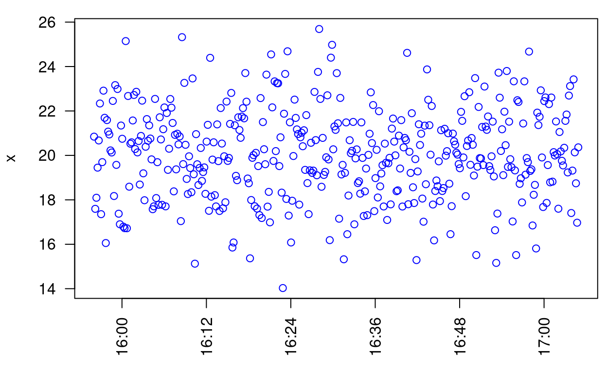

And here’s the same plot using smartTimeAxis(). Notice the intervals are 5 minutes apart, in a natural sequence (i.e., 0, 5, 10, …) as opposed to something less natural (e.g., 2, 7, 12, …):

par(las = 2, mar = c(4, 4, 1, 0.5))

plot(timeData, axes = FALSE, frame.plot = TRUE, xlab = "", col = "Blue")

# Add the y-axis
axis(2)

# Add the time axis
smartTimeAxis(timeData$time, nticks = 20, time.format = "hh:mm")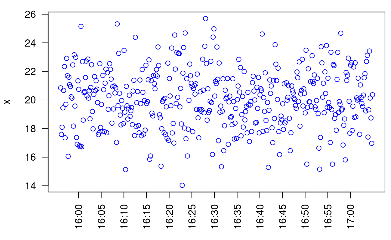

Draw a vertical error bar

vertErrorBar() draws a vertical error bar on a plot, like so:

# Make a plot of some standard normal observations
x <- 1:9
y <- rnorm(9)
plot(x, y, pch = as.character(1:9), ylim = c(-2, 2) + range(y),
     ylab = "Z", xlab = "Indexes")
     
# Draw the error bars
vertErrorBar(x, 0.3, center = y, barLength = 2 * 1.96, blankMiddle = 0.75)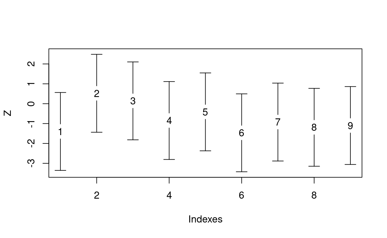

Distribution of the sum of binomials with unequal p

The distribution of the sum of binomial random variates with constant probability of success is well-known. When the probability of sucess varies, things are more complicated. dkbinom() and pkbinom() provide the mass and distribution functions for the sum of an arbitrary number of binomial variates with different success probabilities. Suppose X ~ Bin(5, 0.7) and Y ~ Bin(7, 0.3). Then P(X + Y = 5) is given by:

dkbinom(5, size = c(5, 7), prob = c(0.7, 0.3))

[1] 0.2337159

A continuous version of the binomial cdf

There are circumstances when a continuous version of the discrete binomial cdf can be useful, especially in root finding or optimization. pcbinom() is equivalent to pbinom() when the first argument is an integer.

# These are the same
pcbinom(7, 10, 0.5)

[1] 0.9453125

pbinom(7, 10, 0.5)

[1] 0.9453125

# But these are different
pcbinom(7.5, 10, 0.5)

[1] 0.9739634

pbinom(7.5, 10, 0.5)

[1] 0.9453125

The plot shows how the two functions intersect at the integers

x <- seq(0, 10, length = 500)
y1 <- pbinom(x, 10, 0.5)
y2 <- pcbinom(x, 10, 0.5)
plot(x, y1, type = "s", col = "Blue", xlab = "x", ylab = "F(x)")
lines(x, y2, col = "Red")
legend("topleft", c("pbinom()", "pcbinom()"), lty = 1, col = c("Blue", "Red"))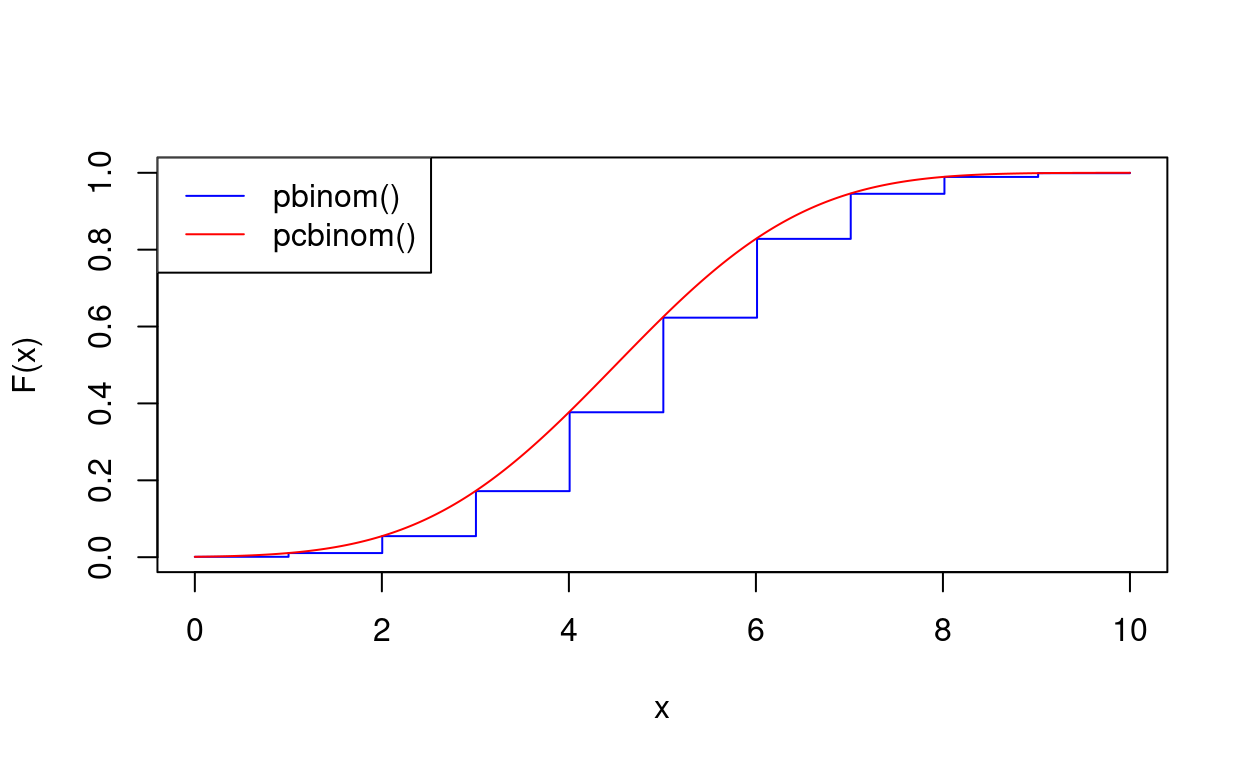

Highest posterior density credible interval

hpd() calculates the highest posterior density (HPD) credible interval for a unimodal density. It requires that we provide a density function, and, if possible, a cdf for the distribution of interest. If the density is expensive to calculate, parallel support is available by simply setting njobs > 1.

Suppose we were interested in making inference about a success probability whose posterior distribution is Beta(7, 20). We could calculate a 95% HPD credible interval as follows:

# The beta pdf and cdf, expressed as functions with a single argument
pdf <- function(x) dbeta(x, 7, 20)
cdf <- function(x) pbeta(x, 7, 20)

# The hpd interval object
hpdInt <- hpd(pdf, c(0, 1), prob = 0.95, cdf = cdf)

# Print the interval
print(hpdInt)

$lower
[1] 0.1056695

$upper
[1] 0.4228501

$prob
[1] 0.9500001

# Plot the interval with the density
plot(hpdInt)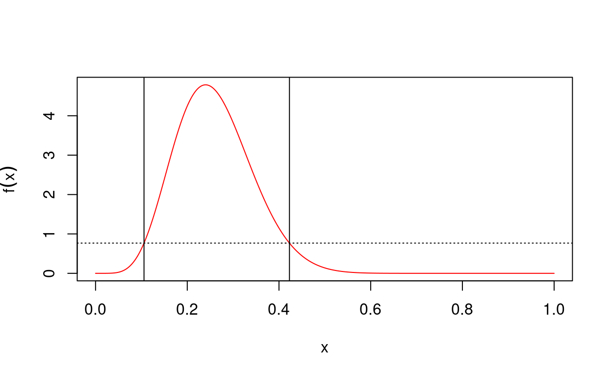

UMVUEs of lognormal parameters

The uniformly minimum variance unbiased estimator (UMVUE) of a lognormal mean is a handful to calculate. umvueLN() calculates the UMVUE of the mean, the standard error of the mean, and the standard deviation of lognormal data, using the formulae presented in Gilbert’s Statistical Methods for Environmental Pollution Monitoring (1987). Here’s a simple example:

# Some lognormal data
x <- exp(rnorm(50, mean = 0.1, sd = 0.5))

# The UMVUE's of the lognormal parameters
umvueLN(x)

        mu      se.mu      sigma 
1.19807880 0.07415374 0.52544544 

Format dates or datetimes

formatDT() makes it easy to convert a vector of dates or datetimes (expressed as character strings) into a variety of formats. A couple of examples:

formatDT("03/12/2004", date.outformat = "dd-mon-yyyy")

$date
[1] "12-Mar-2004"

$time
[1] ""

$dt
[1] "12-Mar-2004"

$date.posix
[1] "2004-03-12 MST"

formatDT("17-Sep-1782 4:31pm", date.outformat = "yyyy-mm-dd", time.outformat = "hh:mm")

$date
[1] "1782-09-17"

$time
[1] "16:31"

$dt
[1] "1782-09-17 16:31"

$dt.posix
[1] "1782-09-17 16:31:00 LMT"

$date.posix
[1] "1782-09-17 LMT"

Calculate a moving window dot product

Have you ever been frustrated by the behavior of filter() near the edges of a time series—or miffed by how it handles NA’s? smartFilter() gracefully handles the beginning and end of a time series, as well as NA’s, by re-normalizing the filter weights as needed. Let’s apply filter() to calculate a moving average consisting of 3 data points:

# A vector
x <- 2^(0:8)
x[4] <- NA
x

[1]   1   2   4  NA  16  32  64 128 256

# The weights
wts <- rep(1, 3) / 3
wts

[1] 0.3333333 0.3333333 0.3333333

# Call filter()
filter(x, wts)

Time Series:
Start = 1 
End = 9 
Frequency = 1 
[1]         NA   2.333333         NA         NA         NA  37.333333  74.666667
[8] 149.333333         NA

And smartFilter() applied to the same data:

smartFilter(x, wts)

[1]   1.500000   2.333333   3.000000  10.000000  24.000000  37.333333  74.666667
[8] 149.333333 192.000000

Moving average with various kernels

movAvg2() will calculate the moving average (i.e. moving dot product) using a 2-sided, symmetric window. Just like smartFilter(), it gracefully handles the edges of time series and NA’s by re-normalizing the weights as needed. The moving window weights can be based on the Gaussian kernel, exponential decay, linear decay, or simple uniform weights.

# Some Gaussian noise
x <- rnorm(50)

# Calculate the moving average using 11 points (bandwidth of 5) 
# and an Gaussian decay kernel:
smooth_x <- movAvg2(x, bw = 5, type = "g")

# Overlay smoothed series on the original data
plot(1:50, x, type = "b", col = "Black", xlab = "Index", ylab = "x")
lines(1:50, smooth_x, col = "Blue", lwd = 3)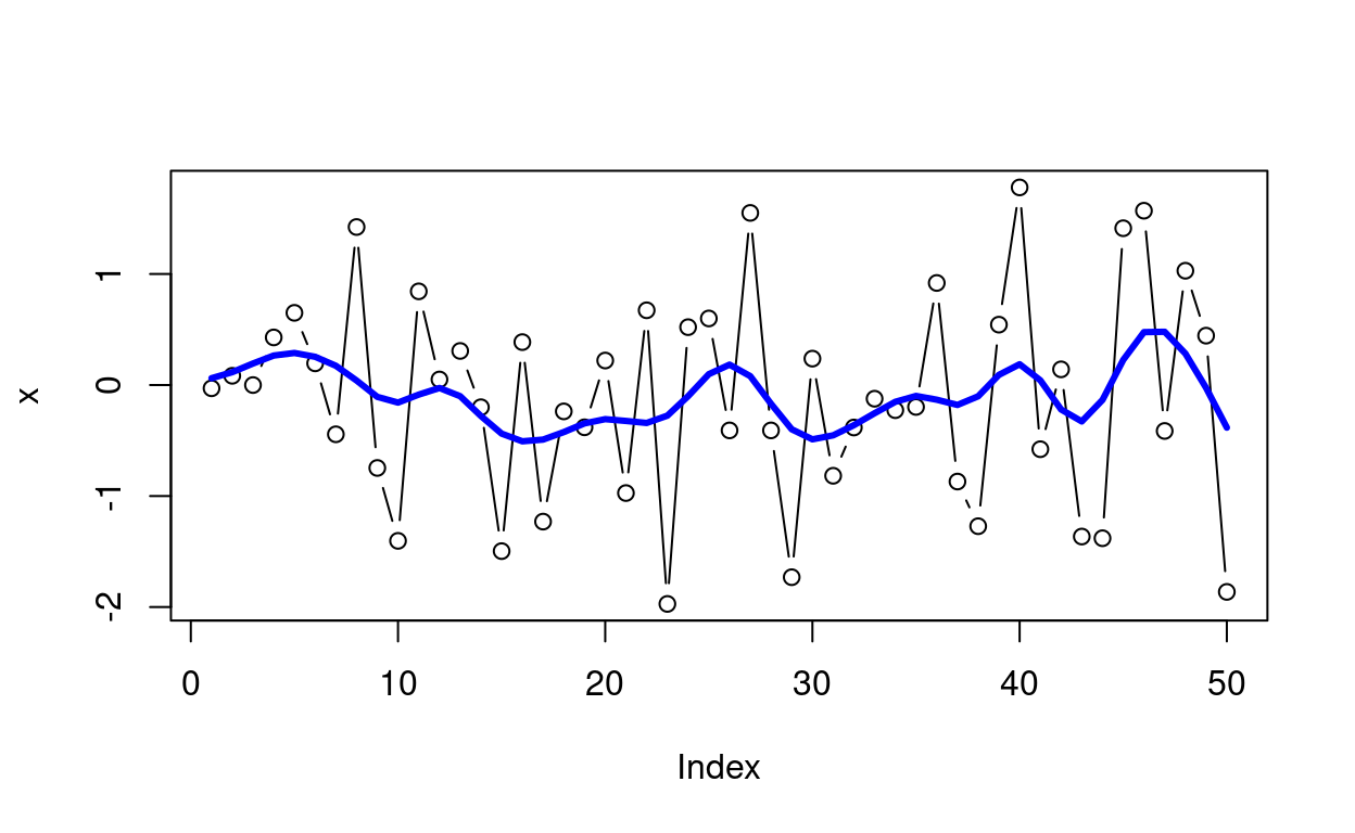

And let’s look at a plot of the weights that we used above:

plot(smooth_x)

Cumulative sum charts (Cusum)

cusum() will calculate the Cusum statistics for a cumulative sum chart of the form C[i] = max(0, C[i − 1] + X[i] − k) that signals when C[i] > h. Here’s a simple example:

# Calculate the Cusum
y <- cusum(rnorm(25), k = 0.2, h = 2)

# Plot results
plot(y, main = "Upper Cusum chart of a standard normal variate", las = 1)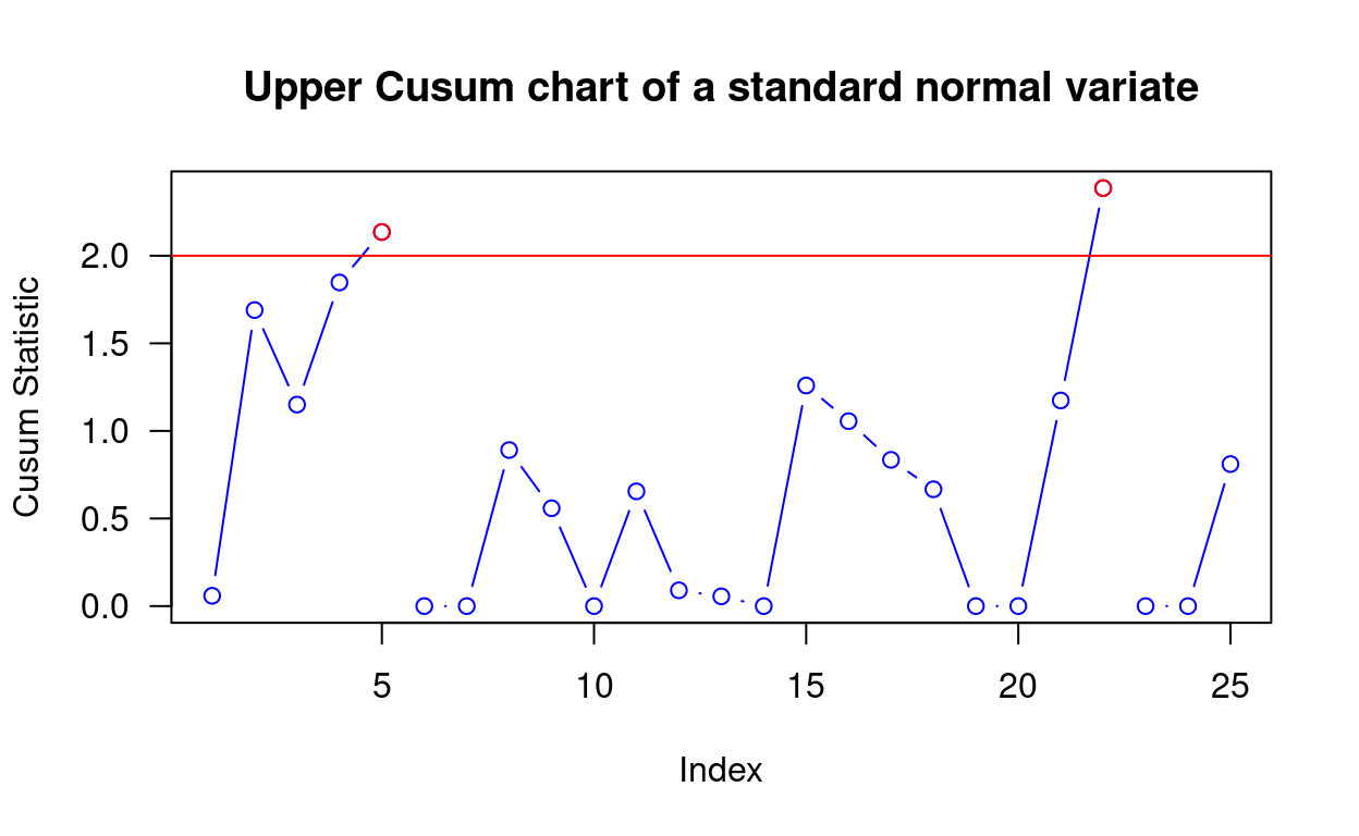

Align two time series

Ever needed to take the difference between two time series that didn’t have matching time indexes? Or have you ever needed to align two time series? timeDiff() can perform both of these functions, even if the series have different lengths or frequencies.

Here are some data. Notice how the two series have different, but roughly similar time stamps:

data(timeDiff.eg)
timeDiff.eg[1:2]

$x1
2009-07-09 10:10:07 2009-07-09 10:10:17 2009-07-09 10:10:27 2009-07-09 10:10:37 
              64.88               65.18               65.11               65.07 
2009-07-09 10:10:47 2009-07-09 10:10:57 2009-07-09 10:11:07 2009-07-09 10:11:17 
              65.14               65.12               64.92               64.95 
2009-07-09 10:11:27 2009-07-09 10:11:37 
              64.97               64.95 

$x2
2009-07-09 10:10:07 2009-07-09 10:10:17 2009-07-09 10:10:27 2009-07-09 10:10:37 
              67.59               67.59               67.63               67.59 
2009-07-09 10:10:49 2009-07-09 10:10:57 2009-07-09 10:11:13 2009-07-09 10:11:20 
              67.65               67.76               67.67               67.74 

We can align them so they have a common set of time stamps:

with(timeDiff.eg, timeDiff(x1, x2, full = TRUE))

        x2.timestamps    original.x1.time original.x1.index    x2    x1
1 2009-07-09 10:10:07 2009-07-09 10:10:07                 1 67.59 64.88
2 2009-07-09 10:10:17 2009-07-09 10:10:17                 2 67.59 65.18
3 2009-07-09 10:10:27 2009-07-09 10:10:27                 3 67.63 65.11
4 2009-07-09 10:10:37 2009-07-09 10:10:37                 4 67.59 65.07
5 2009-07-09 10:10:49 2009-07-09 10:10:47                 5 67.65 65.14
6 2009-07-09 10:10:57 2009-07-09 10:10:57                 6 67.76 65.12
7 2009-07-09 10:11:13 2009-07-09 10:11:17                 8 67.67 64.95
8 2009-07-09 10:11:20 2009-07-09 10:11:17                 8 67.74 64.95
  diff.x1.x2
1      -2.71
2      -2.41
3      -2.52
4      -2.52
5      -2.51
6      -2.64
7      -2.72
8      -2.79

I know the ouput looks a bit bewildering, but the best way to understand how the function aligns the time series is by studying the output of the examples (which are not shown here):

example(timeDiff)

Integration over time

So you have a time series of instantaneous power consumption (in kilowatts) and you need to calculate kilowatt-hours? timeIntegration() will do that quickly for you, illustrating visually how the integral was calculated:

data(PowerData)
timeIntegration(PowerData,
                lower = "5/6/2008 17:00:09",
                upper = "5/6/2008 17:01:36",
                units = "hours",
                check.plot = TRUE)

[1] 0.1247488

More generally, timeIntegration() will approximate the area under any “curve” defined by the linear interpolation of data points, where the units of the domain is time.

Generate all possible combinations

comboList() produces a list that contains all possible combinations of a set of n objects indexed by 1:n. As this can be computationally expensive, it can be easily parallelized with njobs > 1. This extends combn(), which produces all the possible combinations of a specific size. For example, here are all the possible combinations of 3 items, taken 1, 2, and 3 at a time:

out <- comboList(3)
out$pList

[[1]]
[1] 1

[[2]]
[1] 2

[[3]]
[1] 3

[[4]]
[1] 1 2

[[5]]
[1] 1 3

[[6]]
[1] 2 3

[[7]]
[1] 1 2 3

Calculate the maximum up to the current index

For each element of a vector, cumMax() calculates the maximum from the beginning of the vector up to that element.

cumMax(c(1, 2, 3, 0, 2, 4, 1))

[1] 1 2 3 3 3 4 4

Calculate cumulative sum without propagating NA’s

If you need to calculate the cumulative sum of a vector that has missing values, cumsumNA() is your friend. Essentially the same as cumsum(), except it doesn’t propagate NA’s.

x <- c(3, 4, NA, 7, -2)

# cumsum() propagates the NA's
cumsum(x)

[1]  3  7 NA NA NA

# cumsumNA() handles the NA's gracefully
cumsumNA(x)

[1]  3  7 NA 14 12

Identify linearly dependent rows or columns

findDepMat() identifies rows or columns in a numeric matrix that are linearly dependent.

# A matrix
Y <- matrix(c(1, 3, 4, 2, 6, 8, 7, 2, 9, 4, 1, 7, 3.5, 1, 4.5), 
            byrow = TRUE, ncol = 3)

# Note how row 2 is multiple of row 1 and row 5 is a multiple of row 3
print(Y)

     [,1] [,2] [,3]
[1,]  1.0    3  4.0
[2,]  2.0    6  8.0
[3,]  7.0    2  9.0
[4,]  4.0    1  7.0
[5,]  3.5    1  4.5

# Identify rows that are linearly dependent
findDepMat(Y)

[1] FALSE  TRUE FALSE FALSE  TRUE

Numerical integration using Simpson or Trapezoid rule

integ() estimates the integral of a real-valued function using Simpson’s or the Trapezoid approximation. Why might you want something other than integrate()? Because there are occasions when the adaptive quadrature method of integrate() doesn’t behave well—especially if the function is constant over a large portion of the domain.

As a simple example, let’s look at the pdf of a Beta distribution:

f <- function(x) dbeta(x, 5, 5)
plotFun(f, c(0, 1), col = "Blue")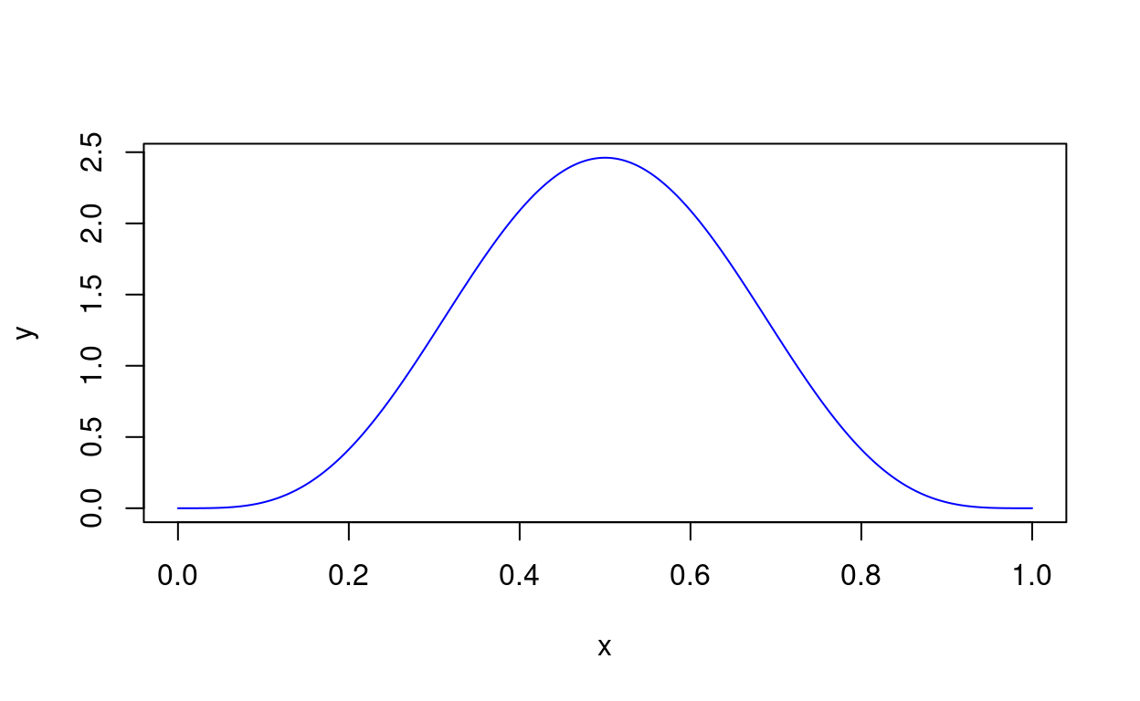

Integration using Simpson’s approximation:

integ(f(seq(0, 0.3, length = 1001)), a = 0, b = 0.3)

[1] 0.09880866

Compare to pbeta():

pbeta(0.3, 5, 5)

[1] 0.09880866

Linear mapping from [a, b] to [c, d]

linearMap() maps a numeric vector or scalar from one closed interval to another. This is especially useful in situations where you want to put multiple variables in the same scale.

# A short sequence in [0, 1]
x <- seq(0, 1, length = 5)
x

[1] 0.00 0.25 0.50 0.75 1.00

# An increasing linear map
linearMap(x, R = c(4, 7))

[1] 4.00 4.75 5.50 6.25 7.00

# A decreasing map
linearMap(x, R = c(7, 4))

[1] 7.00 6.25 5.50 4.75 4.00

# A shift
linearMap(x, R = c(-1, 0))

[1] -1.00 -0.75 -0.50 -0.25  0.00