User Guide

Fundamental Concepts

Basic Methodology

At its most basic level interflow collects input values connecting two sectors in specified units (e.g., water delivered to the agriculture sector), calculates additional sector flows in alternative units based on intensity factors (e.g., energy demand based on water delivered to the agriculture sector), and builds connections to and from additional sectors to carry those values (e.g., electricity sector connected to agriculture sector to deliver the energy)

interflow goes through the following steps in completing calculations:

  1. Collects a Unit 1 “flow” value connecting Node A to Node B

  2. Calculates a Unit 2 value associated with Node B based on a provided Unit 2 per Unit 1 intensity factor for Node B.

  3. Builds a Unit 2 flow value from Node C to Node B as a “source” flow based on the provided fraction of the calculated Unit2 value assumed to come from Node C.

  4. Builds a flow value from Node B to Node D to “discharge” the estimated value based on the provided fraction of the calculated value assumed to go to Node D.

This process is repeated for all nodal relationships within each region provided in the input data.

A real-world example of the above would be:

  1. The total gallons of water withdrawn from the water supply (Node A) and delivered to the public water supply (Node B) is 100 gallons.

  2. The energy required to withdraw a gallon of water from the water supply (Node A) by the public water supply sector (Node B) is 5 british thermal units (btu) per gallon. This calculates out to 500 btu in total based on the initial flow value.

  3. The fraction of energy used in the public water supply sector that is supplied by the electricity sector (Node C) is estimated to be 100%. Therefore, the energy flow value connecting the electricity sector (Node C) to the public water supply sector (Node B) is 500 btu.

  4. The fraction of energy used in the public water supply sector (Node B) that is lost to rejected energy (efficiency losses) is 35%. Therefore, the energy flow value connecting the public water supply sector (Node B) and the rejected energy node (Node D) is 0.35*500 = 175 btu.

The diagram below shows each of these steps.
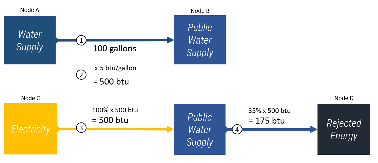
_images/flow_methodology_example.png

Note that interflow does not require node inputs and outputs to be balanced. That is to say, inflows to a node do not have to equal outflows as demonstrated above with only 35% of the energy inflow calculated for public water supply being discharged.

Additionally, while the capability is provided to calculate alternate-unit flows (step 2 above) from input values, this is not a requirement. That is to say, a user could simply provide flow values connecting various nodes in step 1 and the model will simply return those flows unless told to do otherwise.

The example walked through above is a high level example of the flow process that demonstrates what is referred to in this documentation as “level 1” granularity. interflow is capable of calculating and handling sectors up to five levels of granularity. To equate that to the previous example, a level 1 sector would be the public water supply sector. Level 2 and beyond splits up the level 1 sector into subsectors, sub-subsectors, and so on. An example of a level 2 granularity using the above example would be Water Supply - Fresh (i.e., the portion of the total Water Supply sector that is fresh water as opposed to non-fresh water).

Up to five levels of granularity can be specified for each node. Various examples of level 5 granularity include the following:

Level 1

Level 2

Level 3

Level 4

Level 5

Electricity Generation

Natural Gas

Combined Cycle

Carbon Capture Sequestration

Recirculating Cooling

Electricity Generation

Natural Gas

Combined Cycle

Carbon Capture Sequestration

Once Through Cooling

Water Supply

Fresh

Surface Water

Lake

Lake Michigan

More information on generalizability and input data format requirements can be found in the generalizability section.

Aggregation and Output Granularity

While highly granular data can provide significant insight into the finer details of a sector, big picture relationships can also be informative. Though interflow loops through the provided sectors and builds connections at level 5 granularity, it has the capability to aggregate the results to a specified level of granularity. For example, if interflow calculates energy demand in the public water supply sector for public water supply treatment and public water supply distribution, it is capable of returning the total energy in the public water supply (i.e., their sum). Whatever level of granularity is specified (between one and five, inclusive) as a parameter when the model is run will be returned in the output.

Generalizability

Organizing input data

Introduction

Though the interflow package comes with sample data for the US for the year 2015 to calculate water and energy interdependencies, alternative input data can be provided to calculate different flows for any region or set of regions, any unit or set of units, and any sector or set of sectors so long as the input data is provided in the correct format.

The .calculate() function, which is responsible for calculating and organizing the resource flows, requires a Pandas DataFrame with strict guidelines as input data to run calculations. Though different types of calculations are conducted in the interflow package, the data and information used to run each calculation is provided in the same input file.

The four different types of calculations the interflow package conducts include the following:

  1. Collect an input flow value to a primary node from a secondary node in specified units

  2. Calculate an alternative unit flow value based on an intensity factor and the specified primary node flow value

  3. Calculate a source inflow connecting an upstream node to the primary node in the alternative units based on a source fraction

  4. Calculate a discharge outflow connecting the primary node to a downstream node for the alternative units based on a discharge fraction

Each of the above calculation types requires a specific format in the input data that are described in more detail below.

Input data descriptions

The input data for the flow package must have 16 columns described below and each value must be in the column order described below. The interflow package builds a nested dictionary of the input values leading to the various parameter values.

Column #

Description

Type

1

Region

str

2

Calculation type

str

3

Primary Node Level 1 Name

str

4

Primary Node Level 2 Name

str

5

Primary Node Level 3 Name

str

6

Primary Node Level 4 Name

str

7

Primary Node Level 5 Name

str

8

Primary Node Units

str

9

Secondary Node Level 1 Name

str

10

Secondary Node Level 2 Name

str

11

Secondary Node Level 3 Name

str

12

Secondary Node Level 4 Name

str

13

Secondary Node Level 5 Name

str

14

Secondary Node Units

str

15

Parameter

str

16

Value of parameter

flt

Region (columm 1)

The first item in the data should include the name of the region provided as a string. Note that interflow will treat inconsistent spelling of regions as different regions.

Calculation type (columm 2)

The value of the calculation type must equal one of the following verbatim:

  • A_collect

  • B_calculate

  • C_source

  • D_discharge

Each of these inputs tells the model what type of calculation it should be conducting using that row of data.

Primary Node Information (columms 3-8)

Columns 3 through 8 provide information on the primary node (PN). The primary node should be interpreted as the node for which inflows and outflows are determined. Level 1 name refers to the major sector name, Level 2 refers to the sub-sector name, and so on through level 5. For more information on these levels see the Fundamental Concepts section. Primary Node units refers to the resource units (e.g., gallons) that that sector flow name (which will be assigned to a value) is associated with.

Secondary Node Information (columms 9-14)

These data inputs follow the same structure as the primary node but are used to describe the node that is being linked to the primary node as either a source (inflow from),a target node (discharge to), or building a new node to carry an calculated secondary unit value (described in greater detail later on this page).

Parameter (columm 15)

This data item identifies the type of value in the value column (position 16). The value of this data position can be changed by the user with no effect on calculated outcome. It is provided as an optional data position for the user to organize their input data in a more readable manner. Examples (consistent with those in the same data) are shown later on this page.

Value (columms 16)

This data item providing one of the following: (1) an input flow value in primary node units, (2) an intensity coefficient (amount of unit 2 required per unit 1) (3) a source flow fraction, or (4) a discharge flow fraction.

Creating input data for different calculations

Collect values

To build flows between nodes and calculate cross-unit flows, initial flow values are necessary. For example, if the amount of energy required to withdraw a gallon of water from a larger water supply for the public water supply is a desired flow in the ultimate output, then the amount of water withdrawn from the water supply by the public water supply sector is a required input. Initial values must be supplied in the following way:

  • The calculation type (data position 2) must be equal to “A_collect”

  • The primary node information (columns 3-8) must describe the node that is receiving the flow from another node

  • The secondary node information (columns 9-14) must describe the node that is discharging (i.e., upstream) to the primary node

  • The value (column 16) must be equal to value of the flow from the secondary to the primary node

Note that, as shown in the below example, while all data positions must be provided, they do not have to be unique. If there is only level 1 through 3 granularity for some of the input data, the remaining levels can be the same and filled with “total” or an equivalent.

Additionally, some input flow values may be provided that the user does not have a source node for but still wants to calculate secondary unit flows based on. An example might be the production of fuels such as coal. These arguably don’t have a source node when working with water and energy as the two resource types since the coal is the original and most upstream source of the energy, but we may still want to calculate water use based on a water intensity factor for the production of that coal. These values can be provided to the model as circular flows. In this scenario, the primary node information (columns 3-8) will be equal to the secondary node information (columns 9-14). An option is provided in the ‘calculate()’ function to remove circular flows from the output dataframe if desired.

Example:

The below example is collecting a provided flow value equal to 200 mgd that starts from the “Water Supply - Fresh - Surface Water - Total - Total” node and ends at the “Public Water Supply - Fresh - Surface Water - Withdrawal - Total” node

Region

Calculation type

PN L1

PN L2

PN L3

PN L4

PN L5

PN Units

SN L1

SN L2

SN L3

SN L4

SN L5

SN Units

Parameter

value

Region_1

A_collect

Public Water Supply

Fresh

Surface Water

Withdrawal

Total

mgd

Water Supply

Fresh

Surface Water

Total

Total

mgd

flow_value

200

Calculate values

Consistent naming and spelling with sectors is very important as values (both collected and calculated) are assigned to the node names provided. The model looks for node names at level 5 granularity to retrieve known flow values and calculate new flow values based on intensity factors.

In order to calculate secondary unit flow values from collected flow values, the data must be in the following format:

  • The calculation type (column 2) must be equal to “B_calculate”

  • The primary node information (columns 3-8) must describe the new node that is being built in the secondary units (e.g., public water supply pumping energy in btu) based on the intensity factor.

  • The secondary node information (columns 9-14) must describe the node name that the new value is based on and be equal to a node that has already been collected or calculated.

  • The value (column 16) must be equal to the intensity value to calculate the secondary unit flow from the first unit flow. Examples include kilowatt-hours per gallon, gallons per btu, etc.

Note that when calculating a secondary unit flow for a sector that has flows in both units, the names of those sectors/nodes do not have to be consistent as final output values are provided by unit type. In the below example, we are naming the level2 through level5 different than we did for the water flows.

Example:

The example below tells the model to calculate a new energy (bbtu) value and assign it to a new node with a level 5 granularity name of “Public Water Supply - Fresh - Surface Water - Withdrawal - Total” where each dash separates the different granularity levels. The new node and value are being created off of the known level 5 granularity water (mgd) flow value associated with the node name “Public Water Supply - Fresh - Surface Water - Withdrawal - Total”. The intensity factor used to calculate the amount of bbtu per mgd is 2.

Region

Calculation type

PN L1

PN L2

PN L3

PN L4

PN L5

PN Units

SN L1

SN L2

SN L3

SN L4

SN L5

SN Units

Parameter

value

Region_1

B_calculate

Public Water Supply

Fresh

Surface Water

pumping

Total

btu

Public Water Supply

Fresh

Surface Water

Withdrawal

Total

mgd

intensity

2

Note that calculated flow values do not have to be in a secondary unit type. If an intensity value exists that is dependent on the same unit type, the model is capable of handling this. For example, say the amount of water (units = mgd) in the public water supply that was saline was dependent on the the amount of water (units = mgd) in the public water supply that is fresh. So long as a row of data accurately with the intensity factor to determine the saline water quantity in mgd is provided, the model will build it. Additionally, following this example, if a subsequent cross-resource calculation is made on the the total water in public water supply (e.g., energy based on total water), it will base it off the new total water so long as the row to calculate the additional mgd is provided before the row to calculate the energy in the input data.

Source values

Once secondary unit flow values have been calculated by the model, their aggregate value is split into individual flows from various source. For example, if the public water supply sector receives 80% its energy from the electricity sector and 20% from natural gas generators, we would want 80% of our total calculated energy value to be represented as a flow from the electricity node to the public water supply sector and the remaining 20% from the natural gas fuel supply

To split calculated values into sources, the following is required:

  • The calculation type (column 2) must be equal to “C_source”

  • The primary node information (columns 3-8) must describe the node that is receiving the flow from another node (e.g., energy use in public water supply)

  • The secondary node information (columns 9-14) must describe the node that is discharging to the primary node (e.g., electricity sector)

  • The value (column 16) must be the fraction of the calculated value that is coming from the secondary node.

Example:

Region

Calculation type

PN L1

PN L2

PN L3

PN L4

PN L5

PN Units

SN L1

SN L2

SN L3

SN L4

SN L5

SN Units

Parameter

value

Region_1

C_source

Public Water Supply

Fresh

Surface Water

pumping

Total

btu

Electricity Gen.

total

total

total

Total

btu

fraction

.8

Region_1

C_source

Public Water Supply

Fresh

Surface Water

pumping

Total

btu

Fuel Supply

natural gas

total

total

Total

btu

fraction

.2

As many source rows should be provided as there are sources for a particular value. If five nodes feed into a single node, five rows with five fractions that sum to 1 should be provided.

Discharge values

Discharging values follows similar logic as determining source flows in that an aggregate value is split into multiple based on provided fractions. This time, however, the flows being determined are those that are discharged from the primary node (e.g., electricity generation to rejected energy, public water supply to conveyance losses)

To split calculated and collected values into discharges, the following is required:

  • The calculation type (data position 2) must be equal to “D_discharge”

  • The primary node information (data positions 3-8) must describe the node that is discharging the flow to another node

  • The secondary node information (data positions 9-14) must describe the node that is receiving the discharged flow

  • The value (data position 16) must be the fraction of the calculated value that should go to the secondary node.

Example:

Region

Calculation type

PN L1

PN L2

PN L3

PN L4

PN L5

PN Units

SN L1

SN L2

SN L3

SN L4

SN L5

SN Units

Parameter

value

Region_1

C_source

Public Water Supply

Fresh

Surface Water

pumping

Total

btu

Rejected Energy

total

total

total

Total

btu

fraction

.3

Region_1

C_source

Public Water Supply

Fresh

Surface Water

pumping

Total

btu

Energy Services

total

total

total

Total

btu

fraction

.7

As many discharge rows should be provided as there are discharges for a particular value. If one values should be discharged to five downstream nodes, five rows with five fractions that sum to 1 should be provided.

For source and discharge fractions, it is not a strict requirement that the fractions per primary node value sum to one. Note that, not having them sum to 1 will lead to unbalanced flows (greater inflows than outflows or vice versa)

Map Data requirements

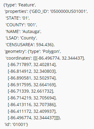
In order to use the optional cloropleth map visualization output that is included in the package, a GeoJSON file containing geometry information for the specified region(s) must be included. The feature.id in the GeoJSON file should match the region column in the output data in order to display correctly. The interflow package comes with a GeoJSON file for US counties, an example of what the GeoJSON file structure looks like is provided below:

_images/json_data_example.png

The image above and the GeoJSON file used for the sample data is part of Plotly’s sample datasets. For more information on the sample GeoJSON file, see the Geospatial section under the US Sample Data Methodology Page.

The cloropleth map output uses the plotly python package. For more information on the GeoJSON input see the GeoJSON with feature.id section within the Plotly cloropleth documentation (https://plotly.com/python/choropleth-maps/)

Key Outputs

Data Outputs

interflow returns a Pandas DataFrame when calling interflow.calculate(). The DataFrame contains the following for each flow value for each region included in the input data when the level parameter is set to 5:

Column Name

Description

Type

region

Name of region

str

S1

Level 1 source node name

str

S2

Level 2 source node name

str

S3

Level 3 source node name

str

S4

Level 4 source node name

str

S5

Level 5 source node name

str

T1

Level 1 target node name

str

T2

Level 2 target node name

str

T3

Level 3 target node name

str

T4

Level 4 target node name

str

T5

Level 5 target node name

str

units

unit type for value

str

value

value of flow connecting source to target

flt

Note that setting the level parameter equal to a value less than 5 will aggregate the output accordingly to the specified levels. For example, specifying level 1 will return the following DataFrame instead.

Column Name

Description

Type

region

Name of region

str

S1

Level 1 source node name

str

T1

Level 1 target node name

str

units

unit type for value

str

value

value of flow connecting source to target

flt

Visualizations

In addition to the Pandas DataFrame output, a variety of visualization and analysis functions are pre-built into the flow package and can be used to interpret results. All visualizations in the package utilize the Plotly open source graphing library. These include the following:

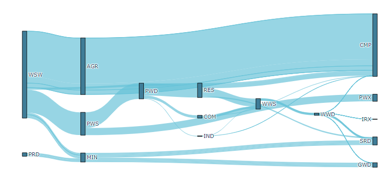
Single-unit sankey diagrams

Sankey diagrams are used to visualize flows from source nodes to target nodes where links between nodes have variable width depending on the value of the flow. The interflow.plot_sankey() function plots up to two sankey diagrams (one for each unit specified) based on the run output that is provided to the function. Users can specify a level of granularity to show flows from level 1 (major sector aggregates only) to level 5 (the highest level of granularity available). For more information on the specific function parameters, defaults, and other components, see the function_guide section.

_images/sankey_example.png

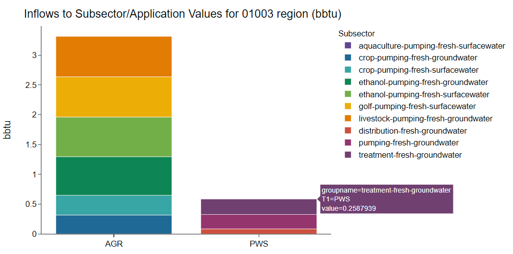
Single region stacked barcharts of sectors

In addition to the Sankey diagrams, there is also the option to plot output in a stacked barchart for any number of sectors. The interflow.plot_sector_bar() function takes a list input of the level 1 sector names (e.g., public water supply) and proceeds to plot inflows or outflows (chosen by the user) into that sector for the specified units. Inflows and outflows are displayed in stacked values of level 5 subsectors within each sector. The barcharts are intended to be used to compare sectors within an individual region for an individual unit.

An example output for energy flows into the agricultural and public water supply sectors for an individual US county from the sample data is shown below.

_images/bar_inflow_example.png

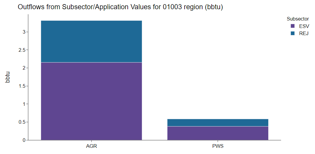
Likewise, the additional figure below shows the energy outflows from those sectors for the same county.

_images/bar_outflow_example.png

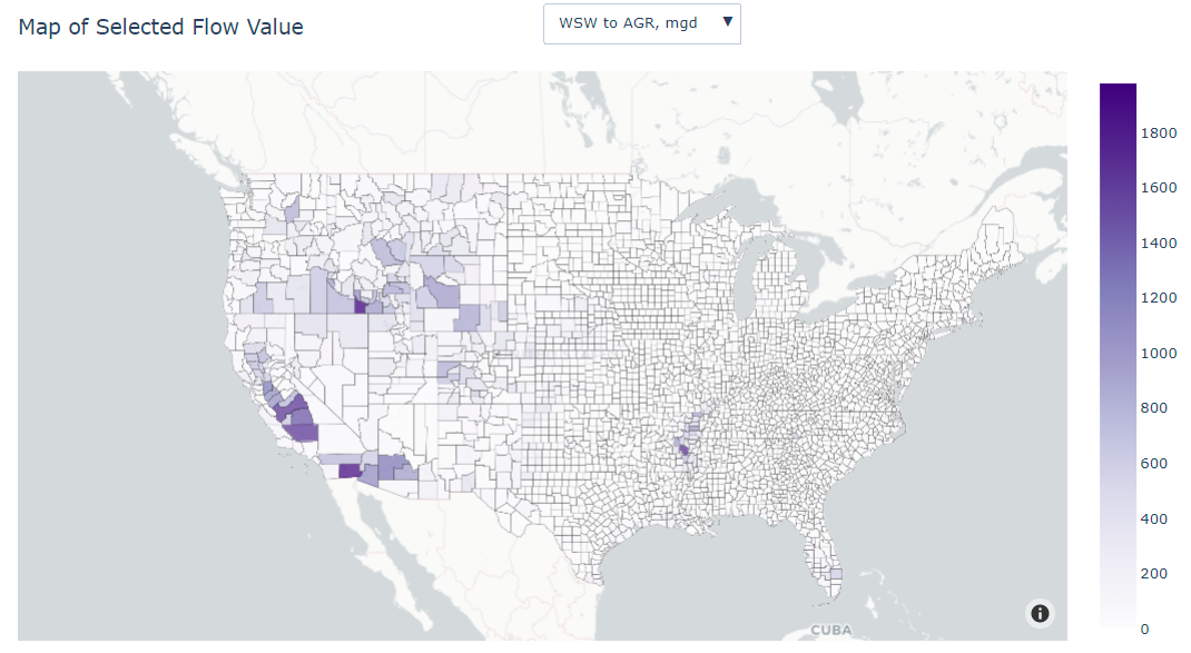
Choropleth map displaying single flow values across regions

The interflow package also comes with the ability to plot flow values on a regional basis. By providing interflow.plot_map() function requires a GeoJSON file to plot a cloropleth map of a selected value. The selectable values are generated as a dropdown list of all available flow values for the specified level of granularity. For example, if level 1 granularity is specified, the drop-down list contains only flows between level 1 nodes. Users can select up to level 5 granularity when running the function and the output will respond appropriately. Below is an example of the cloropleth map output for level 1 granularity for a single flow value using the US county sample data.

_images/map_example.png

Using the Sample Data

Sample data including extensive water and energy data for US counties for the year 2015 is included in the input files folder in the package. This data can be loaded as a pandas DataFrame by running the function ‘.read_sample_data()’. The full sample data is included in the zip file called ‘us_county_sample_data.csv.zip’. The code used to develop this sample data file is included in the sample_data.py module and all input data files used to compile the sample data file are in the input_data folder as well. For more information on the methodology and data sources used to compiles the sample data, see the sample data documentation.