Introduction
Welcome to Hybridlane! Hybridlane is a frontend library for expressing CV-DV quantum circuits, quantum programs that use both qubits and qumodes. Being a frontend library, we focus on providing tools to abstractly describe those circuits independently of the hardware or simulation, and leave the computational heavy-lifting to other libraries.
In this introduction, we’ll briefly cover what Hybridlane does and how to use it with simple examples. These examples will be familiar to Pennylane users, as our library builds on top of it, so we highly recommend reading through the Pennylane documentation as well.
… CV-DV?
Hybridlane implements the so-called “continuous-variable/discrete-variable” (CV-DV) paradigm described by Liu et al (paper). A CV-DV circuit has both discrete variable (DV) components (qubits) and continuous-variable (CV) components (qumodes). As a quick review, the qubits have 2 discrete states, \(\{\ket{0}, \ket{1}\}\), while the qumodes have an infinite number of states corresponding to the quantum harmonic oscillator. Unlike the qubit case, qumodes have two equivalent computational bases: the position basis (\(\{\ket{x}, x\in\mathbb{R}\}\)) and the Fock basis (\(\{\ket{n}, n \in \mathbb{N}_0\}\)). These are linked by the relation
where \(\braket{x|n} = \phi_n(x)\) are the quantum harmonic oscillator eigenstates.
An example
Defining a quantum circuit in Hybridlane follows the same format as Pennylane, and to illustrate this, we’ll show a sample circuit and then walk through the steps.
import numpy as np
import pennylane as qp
import hybridlane as hl

dev = qp.device('default.hybrid', fock_level=8)

@qp.qnode(dev)
def circuit(n):
    for j in range(n):
        qp.X(0)
        hl.JC(np.pi / (2 * np.sqrt(j + 1)), np.pi / 2, [0, 1])

    return hl.expval(hl.N(1))

n = 5
result = circuit(n)
This circuit consists of one qubit (wire 0) and one qumode (wire 1), and it prepares the state \(\ket{0, n}\) by (\(n\) times) pumping one quanta into the qubit and transferring it into the qumode.
Note
In Hybridlane, each circuit starts in the state \(\ket{0\dots 0}\). Differing from the paper, we use the convention that qubits start in their ground state, that is \(\ket{0} = \ket{g} = \ket{\uparrow}\) and \(\ket{1} = \ket{e} = \ket{\downarrow}\). This maintains the conventions used by Pennylane and other mainstream quantum libraries.
Let’s walk through the steps:
import numpy as np
import pennylane as qp
import hybridlane as hl
This code imports both Pennylane (qp) to get access to its decorators and their quantum gates, and our library Hybridlane (hl). Usually you will need both - our library uses all the existing qubit and qumode gates provided by Pennylane, along with extra hybrid (qubit-qumode) gates and utilities provided by us. Pay close attention to which parts use Pennylane functions (qp.) and Hybridlane functions (hl.).
dev = qp.device('default.hybrid', fock_level=8)
When simulating circuits in Pennylane, circuits are usually bound to devices. You must choose a device that supports the operations in your circuit, or you’ll obtain an error (for example, using qp.Displacement gates with the default.qubit device). This line initializes the device registered with name default.hybrid, the default hybridlane simulator.
@qp.qnode(dev)
def circuit(n):
    for j in range(n):
        qp.X(0)
        hl.JC(np.pi / (2 * np.sqrt(j + 1)), np.pi / 2, [0, 1])

    return hl.expval(hl.N(1))
This middle part is the actual circuit definition consisting of its inputs, operation, and outputs (measurements). The special decorator at the top, @qp.qnode(dev), is a Pennylane method for converting pure Python functions into executable quantum circuits. This binds the function circuit to the device dev. Next is our circuit definition, which accepts a single parameter \(n\). The function produces the circuit
Within a circuit definition, you are free to use Python control flow, like loops (for, while) and conditionals (if, else, match). This makes circuits in Pennylane rather flexible. The last argument of a gate (e.g. qp.X or hl.JaynesCummings) is always the “wires”, the qubit(s) and/or qumode(s) that the gate acts on, in order.
The Pauli \(X\) gate (
qp.X) acts on a single qubit and so it accepts a single wire (qubit0)The hybrid qubit-qumode gate \(JC(\theta, \phi)\) (
hl.JaynesCummings) accepts two parameters and then acts on two wires (qumode1and qubit0).
In hybridlane we use the convention that all qubits are listed before qumodes (more on that later).
Tip
You can find the list of gates provided by PennyLane at pennylane. The extra hybrid gates implemented by Hybridlane are at hybridlane. Again, if a class or function is provided under both qp and hl (e.g. NumberOperator, QuadX, expval), use the hl version.
Finally, the return statement determines what measurements our circuit will make. In this case, we obtain the expectation value of the photon number operator on the qumode, \(\braket{\hat{n}_1}\). Here, we use the Hybridlane functions hl.expval and hl.N. Pennylane has its own versions, but we had to redefine them for additional functionality, so use our versions.
Phew that was a lot. But, up until this point (the last two lines), nothing has happened - these are just the definitions. Nothing actually happens until the function circuit is invoked,
n = 5
result = circuit(n)
These lines pass the parameter \(n = 5\) to our circuit, meaning we will prepare the state \(\ket{0, 5}\) and measure its photon number \(\braket{\hat{n}_1} = 5\). Behind the scenes, Pennylane records the operations in our circuit definition, constructs a QuantumTape object, sends it to the device default.hybrid, and returns the result (that’s all the “magic” hidden behind the @qp.qnode decorator).
Tip
At this point you might be wondering how hybridlane determines which wires are qumodes and qubits in a circuit. The short answer is by inspecting the circuit structure and gate definitions, e.g. the wires of a qumode gate are inferred to be qumodes. This is why all our gates enforce the convention that qubits come before qumodes. Inference of the circuit structure is covered more in-depth in the static-analysis section.
Drawing the circuit
PennyLane provides some utility methods for visualizing circuits, pennylane.draw() and pennylane.draw_mpl(), which (mostly) work on Hybridlane circuits.
hl.draw_mpl(circuit, style='sketch')(n)
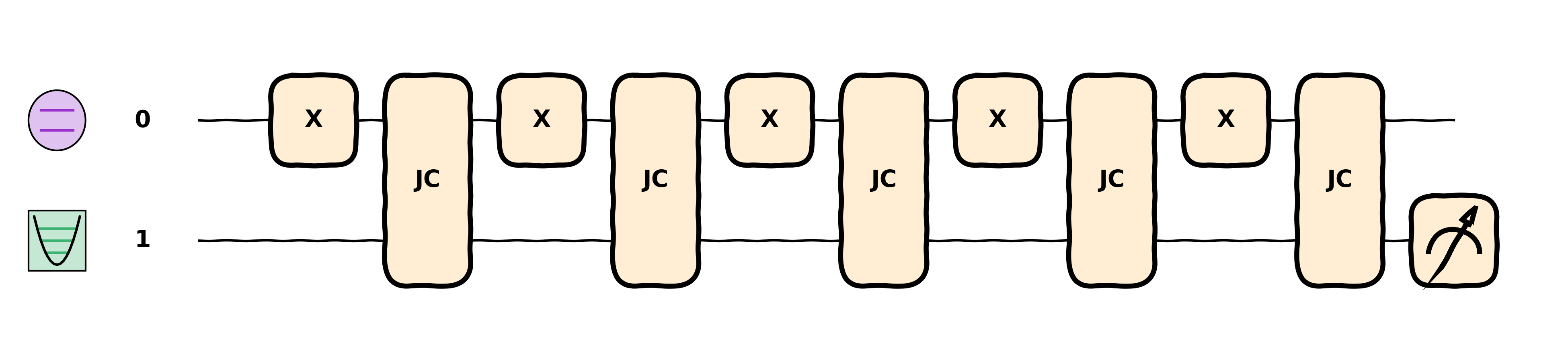
Note that here we use hl.draw_mpl because Hybridlane includes extra functionality to draw
hybrid circuits like support for gates and drawing icons denoting qubits/qumodes.
To view a textual representation of the circuit, we can do
print(qp.draw(circuit)(n))
which produces the output
0: ──X─╭JC(1.57,1.57)──X─╭JC(1.11,1.57)──X─╭JC(0.91,1.57)──X─╭JC(0.79,1.57)──X─╭JC(0.70,1.57)─┤ ···
1: ────╰JC(1.57,1.57)────╰JC(1.11,1.57)────╰JC(0.91,1.57)────╰JC(0.79,1.57)────╰JC(0.70,1.57)─┤ ···

0: ···
1: ···   expval(n̂(1))