A Gentle Introduction to Hypergraph Mathematics

Here we gently introduce some of the basic concepts in hypergraph modeling. We note that in order to maintain this “gentleness”, we will be mostly avoiding the very important and legitimate issues in the proper mathematical foundations of hypergraphs and closely related structures, which can be very complicated. Rather we will be focusing on only the most common cases used in most real modeling, and call a graph or hypergraph gentle when they are loopless, simple, finite, connected, and lacking empty hyperedges, isolated vertices, labels, weights, or attributes. Additionally, the deep connections between hypergraphs and other critical mathematical objects like partial orders, finite topologies, and topological complexes will also be treated elsewhere. When it comes up, below we will sometimes refer to the added complexities which would attend if we weren’t being so “gentle”. In general the reader is referred to [1,2] for a less gentle and more comprehensive treatment.

Graphs and Hypergraphs

Network science is based on the concept of a graph \(G=\langle V,E\rangle\) as a system of connections between entities. \(V\) is a (typically finite) set of elements, nodes, or objects, which we formally call “vertices”, and \(E\) is a set of pairs of vertices. Given that, then for two vertices \(u,v \in V\), an edge is a set \(e=\{u,v\}\) in \(E\), indicating that there is a connection between \(u\) and \(v\). It is then common to represent \(G\) as either a Boolean adjacency matrix \(A_{n \times n}\) where \(n=|V|\), where an \(i,j\) entry in \(A\) is 1 if \(v_i,v_j\) are connected in \(G\); or as an incidence matrix \(I_{n \times m}\), where now also \(m=|E|\), and an \(i,j\) entry in \(I\) is now 1 if the vertex \(v_i\) is in edge \(e_j\).

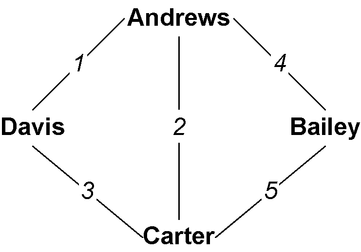
Fig. 1 An example graph, where the numbers are edge IDs.

Table 1 Adjacency matrix \(A\) of a graph.

	Andrews	Bailey	Carter	Davis
Andrews	0	1	1	1
Bailey	1	0	1	0
Carter	1	1	0	1
Davis	1	0	1	1

Table 2 Incidence matrix \(I\) of a graph.

	1	2	3	4	5
Andrews	1	1	0	1	0
Bailey	0	0	0	1	1
Carter	0	1	1	0	1
Davis	1	0	1	0	0

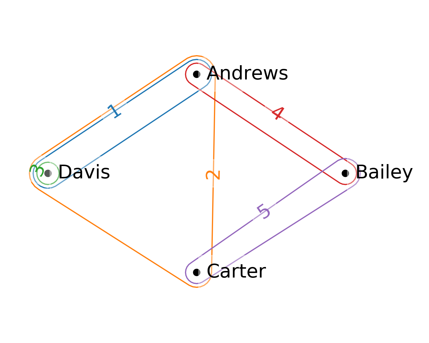
Fig. 2 An example hypergraph, where similarly now the hyperedges are shown with numeric IDs.

Table 3 Incidence matrix I of a hypergraph.

	1	2	3	4	5
Andrews	1	1	0	1	0
Bailey	0	0	0	1	1
Carter	0	1	0	0	1
Davis	1	1	1	0	0

Notice that in the incidence matrix \(I\) of a gentle graph \(G\), it is necessarily the case that every column must have precisely two 1 entries, reflecting that every edge connects exactly two vertices. The move to a hypergraph \(H=\langle V,E\rangle\) relaxes this requirement, in that now a hyperedge (although we will still say edge when clear from context) \(e \in E\) is a subset \(e = \{ v_1, v_2, \ldots, v_k\} \subseteq V\) of vertices of arbitrary size. We call \(e\) a \(k\)-edge when \(|e|=k\). Note that thereby a 2-edge is a graph edge, while both a singleton \(e=\{v\}\) and a 3-edge \(e=\{v_1,v_2,v_3\}\), 4-edge \(e=\{v_1,v_2,v_3,v_4\}\), etc., are all hypergraph edges. In this way, if every edge in a hypergraph \(H\) happens to be a 2-edge, then \(H\) is a graph. We call such a hypergraph 2-uniform.

Our incidence matrix \(I\) is now very much like that for a graph, but the requirement that each column have exactly two 1 entries is relaxed: the column for edge \(e\) with size \(k\) will have \(k\) 1’s. Thus \(I\) is now a general Boolean matrix (although with some restrictions when \(H\) is gentle).

Notice also that in the examples we’re showing in the figures, the graph is closely related to the hypergraph. In fact, this particular graph is the 2-section or underlying graph of the hypergraph. It is the graph \(G\) recorded when only the pairwise connections in the hypergraph \(H\) are recognized. Note that while the 2-section is always determined by the hypergraph, and is frequently used as a simplified representation, it almost never has enough information to be able to recover the hypergraph from it.

Important Things About Hypergraphs

While all graphs \(G\) are (2-uniform) hypergraphs \(H\), since they’re very special cases, general hypergraphs have some important properties which really stand out in distinction, especially to those already conversant with graphs. The following issues are critical for hypergraphs, but “disappear” when considering the special case of 2-uniform hypergraphs which are graphs.

All Hypergraphs Come in Dual Pairs

If our incidence matrix \(I\) is a general \(n \times m\) Boolean matrix, then its transpose \(I^T\) is an \(m \times n\) Boolean matrix. In fact, \(I^T\) is also the incidence matrix of a different hypergraph called the dual hypergraph \(H^*\) of \(H\). In the dual \(H^*\), it’s just that vertices and edges are swapped: we now have \(H^* = \langle E, V \rangle\) where it’s \(E\) that is a set of vertices, and the now edges \(v \in V, v \subseteq E\) are subsets of those vertices.

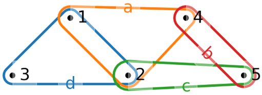
Fig. 3 The dual hypergraph \(H^*\).

Just like the “primal” hypergraph \(H\) has a 2-section, so does the dual. This is called the line graph, and it is an important structure which records all of the incident hyperedges. Line graphs are also used extensively in graph theory.

Note that it follows that since every graph \(G\) is a (2-uniform) hypergraph \(H\), so therefore we can form the dual hypergraph \(G^*\) of \(G\). If a graph \(G\) is a 2-uniform hypergraph, is its dual \(G^*\) also a 2-uniform hypergraph? In general, no, only in the case where \(G\) is a single cycle or a union of cycles would that be true. Also note that in order to calculate the line graph of a graph \(G\), one needs to work through its dual hypergraph \(G^*\).

Fig. 4 The line graph of \(H\), which is the 2-section of the dual \(H^*\).

Edge Intersections Have Size

As we’ve already seen, in a graph all the edges are size 2, whereas in a hypergarph edges can be arbitrary size \(1, 2, \ldots, n\). Our example shows a singleton, three “graph edge” pairs, and a 2-edge.

In a gentle graph \(G\) consider two edges \(e = \{ u, v \},f=\{w,z\} \in E\) and their intersection \(g = e \cap f\). If \(g \neq \emptyset\) then \(e\) and \(f\) are non-disjoint, and we call them incident. Let \(s(e,f)=|g|\) be the size of that intersection. If \(G\) is gentle and \(e\) and \(f\) are incident, then \(s(e,f)=1\), in that one of \(u,v\) must be equal to one of \(w,z\), and \(g\) will be that singleton. But in a hypergraph, the intersection \(g=e \cap f\) of two incident edges can be any size \(s(e,f) \in [1,\min(|e|,|f|)]\). This aspect, the size of the intersection of two incident edges, is critical to understanding hypergraph structure and properties.

Edges Can Be Nested

While in a gentle graph \(G\) two edges \(e\) and \(f\) can be incident or not, in a hypergraph \(H\) there’s another case: two edges \(e\) and \(f\) may be nested or included, in that \(e \subseteq f\) or \(f \subseteq e\). That’s exactly the condition above where \(s(e,f) = \min(|e|,|f|)\), which is the size of the edge included within the including edge. In our example, we have that edge 1 is included in edge 2 is included in edge 3.

Walks Have Length and Width

A walk is a sequence \(W = \langle { e_0, e_1, \ldots, e_N } \rangle\) of edges where each pair \(e_i,e_{i+1}, 0 \le i \le N-1\) in the sequence are incident. We call \(N\) the length of the walk. Walks are the raison d’être of both graphs and hypergraphs, in that in a graph \(G\) a walk \(W\) establishes the connectivity of all the \(e_i\) to each other, and a way to “travel” between the ends \(e_0\) and \(e_N\). Naturally in a walk for each such pair we can also measure the size of the intersection \(s_i=s(e_i,e_{i+1}), 0 \le i \le N\). While in a gentle graph \(G\), all the \(s_i=1\), as we’ve seen in a hypergraph \(H\) all these \(s_i\) can vary widely. So for any walk \(W\) we can not only talk about its length \(N\), but also define its width \(s(W) = \min_{0 \le i \le N} s_i\) as the size of the smallest such intersection. When a walk \(W\) has width \(s\), we call it an \(s\)-walk. It follows that all walks in a graph are 1-walks with width 1. In Fig. 5 we see two walks in a hypergraph. While both have length 2 (counting edgewise, and recalling origin zero), the one on the left has width 1, and that on the right width 3.

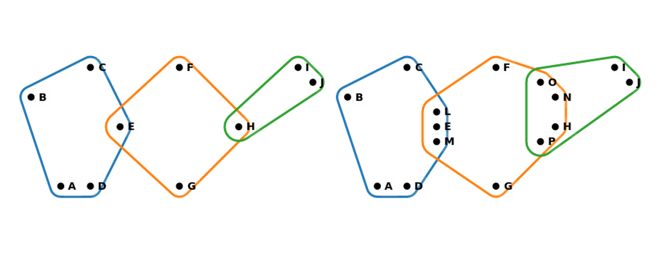
Fig. 5 Two hypergraph walks of length 2: (Left) A 1-walk. (Right) A 3-walk.

Towards Less Gentle Things

We close with just brief mentions of more advanced issues.

\(s\)-Walks and Hypernetwork Science

Network science has become a dominant force in data analytics in recent years, including a range of methods measuring distance, connectivity, reachability, centrality, modularity, and related things. Most all of these concepts generalize to hypergraphs using “\(s\)-versions” of them. For example, the \(s\)-distance between two vertices or hyperedges is the length of the shortest \(s\)-walk between them, so that as \(s\) goes up, requiring wider connections, the distance will also tend to grow, so that ultimately perhaps vertices may not be \(s\)-reachable at all. See [2] for more details.

Hypergraphs in Mathematics

Hypergraphs are very general objects mathematically, and are deeply connected to a range of other essential objects and structures mostly in discrete science.

Most obviously, perhaps, is that there is a one-to-one relationship between a hypergraph \(H = \langle V, E \rangle\) and a corresponding bipartite graph \(B=\langle V \sqcup E, I \rangle\). \(B\) is a new graph (not a hypergraph) with vertices being both the vertices and the hyperedges from the hypergraph \(H\), and a connection being a pair \(\{ v, e \} \in I\) if and only if \(v \in e\) in \(H\). That you can go the other way to define a hypergraph \(H\) for every bipartite graph \(G\) is evident, but not all operations carry over unambiguously between hypergraphs and their bipartite versions.

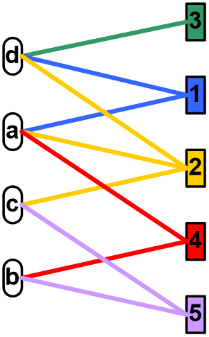
Fig. 6 Bipartite graph.

Even more generally, the Boolean incidence matrix \(I\) of a hypergraph \(H\) can be taken as the characteristic matrix of a binary relation. When \(H\) is gentle this is somewhat restricted, but in general we can see that there are one-to-one relations now between hypergraphs, binary relations, as well as bipartite graphs from above.

Additionally, we know that every hypergraph implies a hierarchical structure via the fact that for every pair of incident hyperedges either one is included in the other, or their intersection is included in both. This creates a partial order, establishing a further one-to-one mapping to a variety of lattice structures and dual lattice structures relating how groups of vertices are included in groups of edges, and vice versa. Fig. refex shows the concept lattice [3], perhaps the most important of these structures, determined by our example.

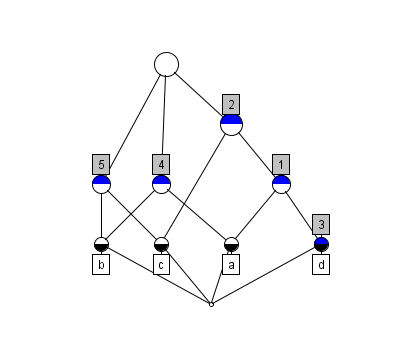
Fig. 7 The concept lattice of the example hypergraph \(H\).

Finally, the strength of hypergraphs is their ability to model multi-way interactions. Similarly, mathematical topology is concerned with how multi-dimensional objects can be attached to each other, not only in continuous spaces but also with discrete objects. In fact, a finite topological space is a special kind of gentle hypergraph closed under both union and intersection, and there are deep connections between these structures and the lattices referred to above.

In this context also an abstract simplicial complex (ASC) is a kind of hypergraph where all possible included edges are present. Each hypergraph determines such an ASC by “closing it down” by subset. ASCs have a natural topological structure which can reveal hidden structures measurable by homology, and are used extensively as the workhorse of topological methods such as persistent homology. In this way hypergraphs form a perfect bridge from network science to computational topology in general.

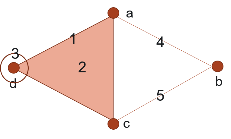
Fig. 8 A diagram of the ASC implied by our example. Numbers here indicate the actual hyper-edges in the original hypergraph \(H\), where now additionally all sub-edges, including singletons, are in the ASC.

Non-Gentle Graphs and Hypergraphs

Above we described our use of “gentle” graphs and hypergraphs as finite, loopless, simple, connected, and lacking empty hyperedges, isolated vertices, labels, weights, or attributes. But at a higher level of generality we can also have:

Empty Hyperedges:

If a column of \(I\) has all zero entries.

Isolated Vertices:

If a row of \(I\) has all zero entries.

Multihypergraphs:

We may choose to allow duplicated hyperedges, resulting in duplicate columns in the incidence matrix \(I\).

Self-Loops:

In a graph allowing an edge to connect to itself.

Direction:

In an edge, where some vertices are recognized as “inputs” which point to others recognized as “outputs”.

Order:

In a hyperedge, where the vertices carry a particular (total) order. In a graph, this is equivalent to being directed, but not in a hypergraph.

Attributes:

In general we use graphs and hypergraphs to model data, and thus carrying attributes of different types, including weights, labels, identifiers, types, strings, or really in principle any data object. These attributes could be on vertices (rows of \(I\)), edges (columns of \(I\)) or what we call “incidences”, related to a particular appearnace of a particular vertex in a particular edge (cells of \(I\)).

[1] Joslyn, Cliff A; Aksoy, Sinan; Callahan, Tiffany J; Hunter, LE; Jefferson, Brett; Praggastis, Brenda; Purvine, Emilie AH; Tripodi, Ignacio J: (2021) “Hypernetwork Science: From Multidimensional Networks to Computational Topology”, in: Unifying Themes in Complex systems X: Proc. 10th Int. Conf. Complex Systems, ed. D. Braha et al., pp. 377-392, Springer, https://doi.org/10.1007/978-3-030-67318-5_25

[2] Aksoy, Sinan G; Joslyn, Cliff A; Marrero, Carlos O; Praggastis, B; Purvine, Emilie AH: (2020) “Hypernetwork Science via High-Order Hypergraph Walks”, EPJ Data Science, v. 9:16, https://doi.org/10.1140/epjds/s13688-020-00231-0

[3] Ganter, Bernhard and Wille, Rudolf: (1999) Formal Concept Analysis, Springer-Verlag