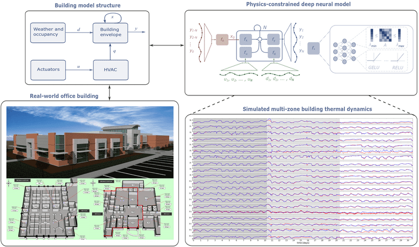
This article summarizes work presented in NeurIPS 2020 Workshop Tackling Climate Change with Machine Learning: Physics-constrained Deep Recurrent Neural Models of Building Thermal Dynamics by Drgoňa, Tuor, Chandan, and Vrabie.

We address the challenge of developing physics-constrained and control-oriented predictive models of the building’s thermal dynamics using a dataset obtained from a real-world commercial building. The proposed method is based on the systematic encoding of the physics-based priors into structured neural architecture with a robust inductive bias towards predicting building dynamics. Specifically, our model mimics the structure of the building thermal dynamics model and leverages penalty methods to model inequality constraints. Additionally, we use constrained matrix parameterization based on the Perron-Frobenius theorem to bind the learned network weights’ eigenvalues. We interpret the stable eigenvalues as dissipativeness of the learned building thermal model. We demonstrate the proposed approach’s effectiveness on a dataset obtained from an office building with 20 thermal zones.

Methods

Physics-based Dynamical Model of Building Thermal Dynamics

In general, the building thermal behavior is determined by high-dimensional, nonlinear and often discontinuous dynamical processes. Thus, obtaining accurate and reliable dynamical models of buildings remains a challenging task and typically involves computationally demanding physics-based modeling. As a consequence, high computational demands and non-differentiability can easily cast the physics-based model not suitable for efficient gradient-based optimization required in various applications. Therefore, a sound trade-off between the model accuracy and simplicity is required.

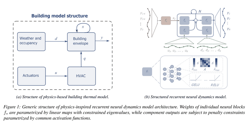
Fortunately, the nature of the building’s dynamics allows us to use several assumptions to decrease the modeling complexity. First, the building envelope model can be accurately linearized around a working point. Second, the HVAC dynamics and weather disturbances can be decoupled from the linearized building envelope dynamics to form a Hammerstein-Wiener model structure illustrated in the following figure 1(a).

These simplifications, allow us to represent the building thermal response model as a following differential equation with non-linear input dynamics:

Where $\bm{x}_{t}$ and $\bm{y}_{t}$ represent the values of the states (envelope temperatures), and measurements (zone temperatures) at time $t$, respectively. Disturbances $\bm{d}_{t}$ represent the influence of weather conditions and occupancy behavior. Heat flows delivered to the building $\bm{q}_{t}$ are defined by mass flows $\dot{\bm{m}}_{t}$ multiplied by a difference of the supply and return temperatures $\Delta \bm{T}_{t}$, and by specific heat capacity $cp$.

If the model is built from physical principles, it is also physically interpretable. For instance, the $A$ matrix represents heat transfer between spatially discretized system states, representing temperatures of the building envelope. $B$ matrix defines the temperature increments caused by the convective heat flow generated by the HVAC system. While, $f_d$ captures the thermal dynamics caused by the varying weather conditions and internal heat gains generated by the occupancy or appliances. However, every building represents a unique system with different operational conditions. Therefore, obtaining the parameters of the above mentioned differential equations from physical principles is a time-consuming, impractical task.

Structured Recurrent Neural Dynamical Model

To incorporate constraints and physics-based structural assumptions, we introduce a generic block nonlinear state space model (SSM) for partially observable systems. Each block of this structured graph model corresponds to a different part of the generic building model structure. Thus the overall physically interpretable architecture is shown in figure 1(b). The block-structured recurrent neural dynamics model is then defined as:

Here $f_{x}$, $f_{u}$, and $f_{d}$ represent decoupled neural components of the overall system model. The advantage of the block nonlinear over black-box state space model lies in its structure. The decoupling allows us to leverage prior knowledge for imposing structural assumptions and constraints onto individual blocks $f_*$ of the model.

Constraining Eigenvalues of the System Dynamics

One key physics insight is that building thermal dynamics represents a dissipative system with stable eigenvalues. This inspired us to enforce physically reasonable constraints on the eigenvalues of a model’s weight matrices. We leverage the method based on the Perron-Frobenius theorem, which states that the row-wise minimum and maximum of any positive square matrix define its dominant eigenvalue’s lower and upper bound, respectively. Guided by this theorem, we can construct a state transition matrix $\bm{\tilde{A}}$ with bounded eigenvalues:

We introduce a matrix $\bm{M}$ which models damping parameterized by the matrix $\bm{M'} \in \mathbb{R}^{n_x \times n_x}$. We apply a row-wise softmax to another parameter matrix $\bm{A'} \in \mathbb{R}^{n_x \times n_x}$, then elementwise multiply by $\bm{M}$ to obtain our state transition matrix $\bm{\tilde{A}}$ with constrained eigenvalues in the interval $(1 - \epsilon, 1)$.

Inequality Constraints via Penalty Methods

Using an optimization strategy known as the penalty method, we can add further constraints to our model such that its variables remain within physically realistic bounds. We use a simple method for enforcing this property by applying inequality constraints via penalty functions $p(\bm{x})$ for each time step $t$:

The constraints lower and upper bounds are given as $\bm{\underline{y}}_k$ and $\mathbf{\overline{y}}_k$, respectively. The slack variables $\bm{s}^{\underline{y}}_k$ and $\bm{s}^{\overline{y}}_k$ indicate the magnitude to which each constraint is violated, and we penalize them heavily in the optimization objective by a large weight on these additional terms in the loss function.

Multi-term Loss Function

Now everything comes together in a weighted multi-term loss function. We optimize the following loss function augmented with regularization and penalty terms to train the recurrent neural model unrolled over $N$ steps:

The main objective of loss function computes the mean squared error between predicted $\bm{y}$ and observed outputs $\bm{y}^{\text{ref}}$ over $N$ time steps. The term $\bm{x}_{t} - \bm{x}_{t-1}$ represents state difference penalty promoting learning of smoother and physically more plausible state trajectories. The violations of inequality constraint defining the boundary conditions of outputs $\bm{y}$ is penalized by incorporating weighted slack variables $\bm{s}^{\bm{y}}$. Thanks to the block-structured dynamics, we can constrain the dynamical contribution of inputs $f_u$ and disturbances $f_d$ towards the overall dynamics via two additional terms in the loss function. This allows us to limit the effect of the external factors to be bounded within physically plausible ranges. For instance, it is not physically realistic that $1K$ change in the ambient temperature would result in $2K$ change in indoor temperature in a single time step.

Experimental Case Study

Dataset

The objective is to develop a control-oriented thermal dynamics model of a commercial office building, given a limited amount of measurement data. The building used in this study is a commercial office building with $20$ thermal zones. Heating and cooling are provided by a variable air volume (VAV) system served by $4$ air handling units (AHUs) serving $24$ VAV boxes (zones). Each VAV box is equipped with a hot water reheat coil. A boiler, fed by natural gas, supplies hot water to the reheat coils and AHU coils. Chilled water is supplied by a central chiller plant.

The time series dataset $D$ is given in the form of tuples with input, disturbance, and output variables, respectively.

where $i = \bm{N}_1^n$ represents index of $n$ batches of time series trajectories with $N$-step horizon. The data is sampled with sampling time $\Delta = 15$ min. We have in total $n_y = 20$ output variables corresponding to zone temperatures, $n_u = 40$ input variables representing HVAC temperatures and mass flows, and $n_d = 1$ disturbance variable for ambient temperature forecast. We use \texttt{min-max} normalization to scale all variables between $[0, 1]$. The dataset consists of $30$ days, which corresponds to only $2880$ datapoints. We group the dataset into evenly split training, development, and test sets, $960$ data points each.

Experimental Setup

We implement the models using Pytorch, and train with randomly initialized weights using the Adam optimizer with a learning rate of $0.003$, and $5,000$ gradient descent updates. We select the best performing model on the development set, and report results on the test set. The state estimator $f_o$ is a fully connected neural network, while neural blocks $f_*$ are represented by recurrent neural networks with $2$ layers and $80$ nodes. We range the prediction horizon as powers of two $2^n$ with $n = 3, \ldots, 6$, which corresponds to $2$ up to $16$ hour window. The relative weights of the multi-term loss function are $Q_{\text{dx}}=0.2$, $Q_{\text{ineq}}^{\mathbf{y}}=1.0$, $Q_{\text{ineq}}^{\mathbf{u}}=0.2$, and $Q_{\text{ineq}}^{\mathbf{d}}=0.2$. We set $\lambda_{\text{min}} =0.8$ and $\lambda_{\text{max}}=1.0$ for stability and dissipativity of learned dynamics.

Results and Analysis

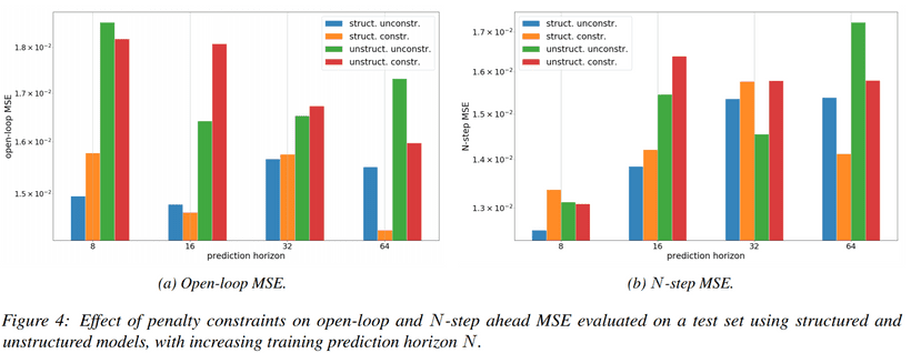
We assess the simulated open-loop and $N$-step MSE performance of the recurrent model with and without physics-constraints and structure. The MSE metrics are shown in figure 4 and in following table.

The open-loop MSE of the best-performing constrained and structured model corresponds to $0.488$K. In comparison, the state of the art gray-box system identification methods trained on a similar amount of data reports open-loop MSE roughly equal to $1.0$K. Hence our preliminary results show more than $50\%$ reduction in error against state of the art in literature. We observe that imposing physics-inspired structure and constraints not only yields $15\%$ reduction of error but allows us to train models with a larger prediction horizon $N$. The performance of the best-performing models is compared in the following figures and table.

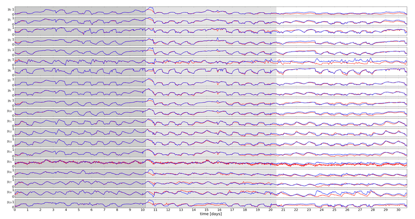
We perform dynamical simulation of the learned dynamical model by unrolling its dynamics into the future. By comparing the trajectories against measured data, we demonstrate the capability to generalize complex dynamics over $30$-days using only $10$-days of training data.

Eigenvalue Analysis and Physical Interpretability

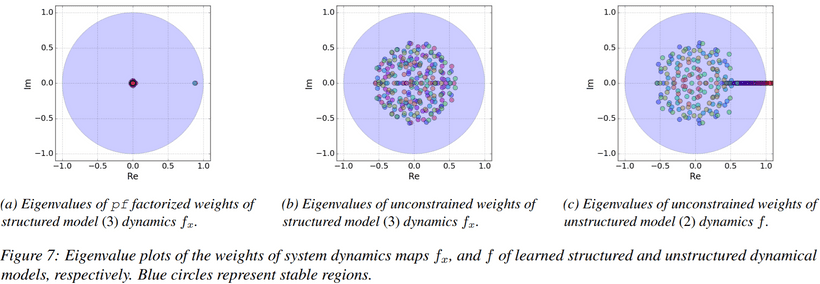
Now we show how using eigenvalue constraints promotes physical coherence and interpretability of the learned model. Following figure 7 shows concatenated eigenvalues in the complex plane for weights of the state transition maps $f_x$ with and without eigenvalue constraints. We also compare the eigenvalues of the classical unstructured recurrent neural model which lumps the building dynamics into a single block $f$. Please note that we plot only eigenvalues of the neural network’s weights. Hence the dynamic effects of the activation functions are omitted in this analysis. However, all our neural network blocks are designed with GELU activation functions, which represent contractive maps with strictly stable eigenvalues. Therefore, based on the argument of the composition of stable functions, the global stability of the learned dynamics is not compromised.

Figure 7(a) shows the effect of proposed Perron-Frobenius factorization, and verifies that the dominant eigenvalue remains within prescribed bounds $\lambda_{\text{min}} =0.8$ and $\lambda_{\text{max}}=1.0$. Hence the disipativeness of the learned dynamics is hard constrained within physically realistic values when using eigenvalue constraints. Another interesting observation is that there are only two dominant dynamical modes with eigenvalues larger than $0.8$, one per each layer of $f_x$. While the rest of the eigenvalues fall within $0.05$ radius, hence representing less significant dynamic modes. This indicates a possibility to obtain lower-order representations of the underlying higher-order nonlinear system, a property useful for real-time optimal control applications. On the other hand, as shown in figure 7(c), using a standard recurrent model with lumped dynamics results in losing physical interpretability and generates physically implausible unstable dynamical modes violating the disipativeness property. Moreover, the imaginary parts of unconstrained dynamics shown in figure 7(b) and 7(c) indicate oscillatory modes of the autonomous state dynamics. However, in the case of building thermal dynamics, the periodicity of the dynamics is caused by external factors such as weather and occupancy schedules. From this perspective, the structured models using eigenvalue constrained weights are closer to the physically realistic system dynamics.

Conclusion

Reliable data-driven methods that are cost-effective in terms of computational demands, data collection, and domain expertise have the potential to revolutionize the field of energy-efficient building operations through the wide-scale acquisition of building specific, scalable, and accurate prediction models. We presented a constrained deep learning method for sample-efficient and physics-consistent data-driven modeling of building thermal dynamics. Our approach does not require the large time investments by domain experts and extensive computational resources demanded by physics-based emulator models. Based on only 10 days’ measurements, we significantly improve on prior state-of-the-art results for a modeling task using a real-world large scale office building dataset. A potential limitation of the presented approach is the restrictiveness of the used constraints, where wrong initial guess of the eigenvalue and penalty constraints bounds may lead to decreased accuracy of the learned model. Future work includes a systematic comparison against physics-based emulator models and other standard data-driven methods. Authors also plan to use the method as part of advanced predictive control strategies for energy-efficient operations in real-world buildings.

Acknowledgement

This research was supported by the Laboratory Directed Research and Development (LDRD) at Pacific Northwest National Laboratory (PNNL). PNNL is a multi-program national laboratory operated for the U.S. Department of Energy (DOE) by Battelle Memorial Institute under Contract No. DE-AC05-76RL0-1830.