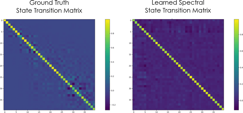
This article summarizes work presented in Constrained Neural Ordinary Differential Equations with Stability Guarantees by Tuor, Drgoňa, and Vrabie.

Comparison of ground truth and learned, spectrally-constrained system state transition matrices for a multi-input multi-output dynamical system. Learned state dynamics are parameterized by our neural ODE model.

Ordinary differential equations are broadly applicable to numerous problems in the engineering domain, and are often employed for the modeling and control of industrial systems. However, traditional physics-based modeling of dynamical systems often requires domain expertise, may be computationally prohibitive for more complex systems, and may prove difficult to adapt to new systems. This work proposes a novel approach to modeling discrete ODEs with algebraic nonlinearities using neural networks. This is accomplished by embedding the physical characteristics and behaviors of dynamical systems directly into neural networks as structural priors and inequality constraints. This unification of physics-based and data-driven modeling approaches allows for varying degrees of prior knowledge to be incorporated into dynamical models, yielding more robust models with less data.

From State Space Models to Neural ODEs

State space models for dynamical systems can take numerous forms according to the real-world characteristics of a system. As a case study, consider the following linear time-invariant state space model with input nonlinearity, otherwise known as a Hammerstein model:

\begin{aligned} \bm{x}_{k+1} &= \bm{Ax}_k + \bm{Bu}_k + \bm{Ed}_k \\ \bm{u}_k &= \bm{a}_k\bm{Hb}_k + \bm{h} \end{aligned}

where $\bm{x}_k$ is the system state, $\bm{u}_k$ is the system input, and $\bm{d}_k$ is disturbance at time $k$ . In this example, the system input $\bm{u}_k$ is given as an algebraic equation which expresses a bilinear interaction between input terms $\bm{a}_k$ and $\bm{b}_k$ modeled by the coefficients $\bm{H}$ and $\bm{h}$ , though in practice this could be any time-invariant nonlinear equation.

Notice that the first equation shown above is a discrete ordinary differential equation describing the evolution of the system’s state over time. We can translate this discrete ODE into a structured recurrent neural network which similarly describes this state evolution as transitions between the RNN’s hidden states forward in time:

\begin{aligned} \tilde{\bm{x}}_{t+1} &= f(\tilde{\bm{A}}\tilde{\bm{x}}_t + \tilde{\bm{B}}\bm{u}_t + \tilde{\bm{E}}\bm{d}_t) \\ \bm{u}_t &= h_{\Theta}(\bm{a}_t, \bm{b}_t). \end{aligned}

Here, we generalize the input bilinearity as some function $h_{\Theta}$ ; this allows us to define the system’s input according to varying degrees of prior knowledge of the algebraic equation determining the system’s input. For instance, if we had no prior knowledge of the underlying bilinear structure or parameters of our system’s input equation, we could let $h_{\Theta}$ be some function with arbitrary structure and learnable parameters, i.e. a fully-connected neural network. Although useful for modeling systems with complex or unknown physical properties, this black-box approach has the drawback of poorer sample efficiency and interpretability.

If we did happen to know the bilinear structure of $h_{\Theta}$ , but not necessarily its parameters, we could simply embed the same algebraic structure into $h_{\Theta}$ and learn the parameters of the equation as we would in the previous black-box case:

\begin{aligned} h_{\Theta}(\bm{a}_t, \bm{b}_t) &= \bm{a}_t\tilde{\bm{H}}\bm{b}_t + \tilde{\bm{h}} \\ \Theta &= \{\tilde{\bm{H}}, \tilde{\bm{h}}\} \end{aligned}

This grey-box approach has the advantage of reducing the complexity of learning the input’s true parameters by constraining the space of possible functions which can be approximated by $h_{\Theta}$ . This property can improve data efficiency considerably; with fewer parameters, these models can more effectively learn from fewer observations of the ground-truth system.

Of course, if we knew not only the algebraic structure of $h_{\Theta}$ but also its parameters, we can take the white-box approach of specifying both directly and avoid any guesswork on the structure or parameters of the input function entirely.

This state space model is just one example out of many possible variations that can be accommodated by this neural ODE formulation.

Adding Constraints for Stability and Realism

Dynamics Stability via Eigenvalue Constraints

Because dynamical models are often used in real-world, safety-critical contexts, verifying their stability is crucial. Fortunately, research on measuring the stability of deep neural networks has led some researchers to study and analyze deep models through the lens of dynamical systems, providing domain-relevant insight we can incorporate into our neural state space models. An example of this is Haber and Ruthotto’s Stable Architectures for Deep Neural Networks, which establishes that imposing certain constraints on the parameters of deep neural networks can provide stability guarantees for both forward and backward propagation.

One key insight is in constraining the eigenvalues of a model’s weight matrices. We refer to the Perron-Frobenius theorem, which states that the row-wise minimum and maximum of any positive square matrix defines its dominant eigenvalue’s lower and upper bound, respectively. Guided by this theorem, we can construct a state transition matrix $\bm{\tilde{A}}$ with bounded eigenvalues:

\begin{aligned} \bm{M} &= 1 - \epsilon\sigma(\bm{M'}) \\ \bm{\tilde{A}}_{i,j} &= \frac{\text{exp}(\bm{A'}_{ij})}{\sum_{k=1}^{n_x} \text{exp}(\bm{A'}_{ik})}\bm{M}_{i,j} \end{aligned}

First, we introduce a matrix $\bm{M}$ which models damping parameterized by the matrix $\bm{M'} \in \mathbb{R}^{n_x \times n_x}$ . We apply a row-wise softmax to another parameter matrix $\bm{A'} \in \mathbb{R}^{n_x \times n_x}$ , then elementwise multiply by $\bm{M}$ to obtain our state transition matrix $\bm{\tilde{A}}$ with constrained eigenvalues in the interval $(1 - \epsilon, 1)$ .

Optimization with Inequality Constraints

Using an optimization strategy known as the penalty method, we can add further constraints to our model such that its variables remain within physically realistic bounds. We use a simple method for enforcing this property by applying inequality constraints for each time step $k$ :

\begin{aligned} \bm{\underline{x}}_k \leq \bm{x}_k + \bm{s}^{\underline{x}}_k \:\:\: &\cong \:\: \bm{s}^{\underline{x}}_{k} = \text{max}(0,\:-\bm{x}_k + \bm{\underline{x}}_k) \\ \bm{x}_k - \bm{s}^{\overline{x}}_k \leq \bm{\overline{x}}_k \:\:\: &\cong \:\: \bm{s}^{\overline{x}}_{k} = \text{max}(0,\:\bm{x}_k - \bm{\overline{x}}_k) \end{aligned} \\

Looking at the left-hand sides of these congruences, we first define inequality constraints for the model’s state vector $\bm{x}$ . These constraints are given as $\bm{\underline{x}}_k$ and $\bm{\overline{x}}_k$ , which correspond to the model state’s lower and upper constraints, respectively. The magnitude of the slack variables $\bm{s}^{\underline{x}}_k$ and $\bm{s}^{\overline{x}}_k$ tells us the degree to which each constraint is violated.

To understand how this translates to state value constraints, let’s first look at the upper-bound constraint. Notice that if the difference between the state and its upper bound is positive, then the state value must exceed the bound. Otherwise, if the result is negative, the state must be within bounds and the constraint satisfied. To avoid penalizing the model in the latter case, we zero out any negative values, finally obtaining the upper bound slack variable. The same algebraic intuition can be applied to our lower-bound constraint to obtain the value of its corresponding slack variable.

By teasing apart the inequalities we started with, we obtain equivalent boundary functions we can use in the model’s loss function to enforce inequality constraints during training. Such inequality constraints can be devised for any variables in the system in accordance with their known physical bounds.

Training the Neural ODE Model

Putting together our structured RNN with parameter eigenvalue constraints and inequality constraints, we now define a loss function to be used with gradient descent and backpropagation to train the model:

\mathcal{L}_{\text{MSE}}(\mathcal{\tilde{X}}, \mathcal{X} | \bm{\tilde{A}}, \bm{\tilde{B}}, \bm{\tilde{E}}, \Theta) = \frac{1}{N} \sum_{k=1}^{N} ((\bm{\tilde{x}}_{k,i} - \bm{x}_{k,i})^2 + \lambda(\bm{s}^{x}_{k})^2 + \mu(\bm{s}^{u}_{k})^2)

At a high level, the loss function computes mean squared error between predicted and ground truth state value observations over $N$ time steps, while incorporating weighted slack variables as boundary functions to penalize inequality constraint violations during training.

Breaking it down further, $\mathcal{X} = \bm{x}_0, \dots, \bm{x}_N$ corresponds to ground-truth system state observations from a data set obtained by simulating a ground truth system equation over $N$ time steps—in this case, the Hammerstein block model introduced previously. Also included in the data set are system input sequences $\mathcal{A}$ and $\mathcal{B}$ , as well as disturbances $\mathcal{D}$ . These sequences along with initial ground truth state $\bm{x}_0$ are then given to the model to produce a sequence of predicted system states $\mathcal{\tilde{X}}$ .

Computing the squared error between ground-truth and predicted states then yields the model’s deviation from the ground truth model. This is combined with joint slack variables which combine lower and upper constraints for system components into single variables: $\bm{s}^x_k = \bm{\underline{s}}^x_k + \bm{\overline{s}}^x_k$ constrains system state, and $\bm{s}^u_k$ is similarly defined to constrain system input. The loss function weights these slack terms with hyperparameters $\lambda$ and $\mu$ to specify the degree of penalization incurred by each term.

Finally, the loss is defined to optimize the parameters $\bm{\tilde{A}}$ , $\bm{\tilde{B}}$ , and $\bm{\tilde{E}}$ used by our structured neural ODE. The $\Theta$ parameters can also be optimized for the black-box and grey-box cases previously described. As mentioned, we apply gradient descent with backpropagation to learn the unknown parameters of the model in a data-driven manner.

Experiments

To validate our proposed approach to dynamic system identification, we evaluate our models with and without inequality constraints (hereafter referred to as cODE and ODE), and evaluate both of those variants under the three degrees of prior knowledge described previously (ODE_B for black-box models, ODE_G for grey-box, and ODE_W for white-box).

Target Dynamics

Using the Hammerstein model with which we established our case study, we validate our model by simulating a building thermal system. The system state $x \in \mathbb{R}^4$ contains components for wall ( $x_1$ ), ceiling ( $x_2$ ), floor ( $x_3$ ), and ambient room ( $x_4$ ) temperatures. We assume that our single observable variable is ambient room temperature.

The bilinear input term used by the model is a heat flow equation with a constant parameter of specific heat capacity $\bm{H} = c_p$ , $\bm{h} = 0$ and two variables: mass flow $\bm{a}_k = \bm{\dot{m}_k}$ and difference of supply and return temperature $\bm{b}_k = \Delta\bm{T}_k$ . Control inputs $\mathcal{A}$ and $\mathcal{B}$ are given as sine and cosine waves, respectively, with 24-hour periods and amplitudes matching values typical of actual control inputs to the ground-truth model. Finally, the disturbance signal $\mathcal{D}$ represents historical environmental conditions. We split the data set into train, validation, and test sets using the 2^nd, 3^rd, and 4^th weeks of simulation, respectively, leaving each split with 2016 contiguous samples.

Model Training Procedure

For all the models mentioned previously, we train each using the $N$ -step prediction objective defined earlier. Each model is trained with $N \in \{2^3, \dots, 2^7\}$ , and for each $N$ we train 30 models with randomly-initialized parameters. Model parameters are learned with full-batch gradient descent for 15,000 epochs using AdamW at learning rates ranging from 0.001 to 0.03. Models are evaluated on both their $N$ -step training objective and open-loop mean squared error for model simulation over the test set.

Results and Analysis

	$N$ -Step Prediction Error						Open-Loop Prediction Error
N	8	16	32	64	128		8	16	32	64	128
ODE_B ODE_G ODE_W cODE_B cODE_G cODE_W	0.04 0.08 0.08 0.03 0.08 0.08	0.13 0.33 0.31 0.13 0.33 0.33	0.47 0.92 0.92 0.46 0.92 0.92	0.31 0.82 0.81 0.30 0.91 0.82	0.41 0.65 0.65 0.35 0.58 0.59		9.93 19.0 19.6 3.44 19.5 19.9	3.75 23.0 19.2 3.48 19.5 19.6	5.15 4.19 6.58 4.94 4.68 6.91	2.24 0.91 5.24 2.47 2.96 7.60	2.59 2.56 3.81 0.22 0.56 0.41

Table 1: Best-observed test set mean squared errors for N-step and open-loop predictions.

As indicated by Table 1, increasing the prediction horizon increases the error of $N$ -step predictions, yet lowers that of open-loop predictions; as we increase the $N$ -step prediction horizons used during training, we presumably obtain increasingly better approximations to the open-loop behavior of the models, yielding better performance. This increase in open-loop performance is especially noticable for each of the constrained models. However, the same cannot be said of the unconstrained black- and grey-box models, whose performance drops upon reaching the maximum prediction horizon.

The best performing model was the constrained black-box model cODE_B, despite lacking any priors over the algebraic structure of the model. This result suggests that given prior knowledge of a system’s physical constraints, accurate models can be obtained without full prior knowledge of the ground-truth system’s underlying algebraic structure or parameters.

Figure 2: Open-loop trace analysis for non-constrained (left) and constrained (right) models.

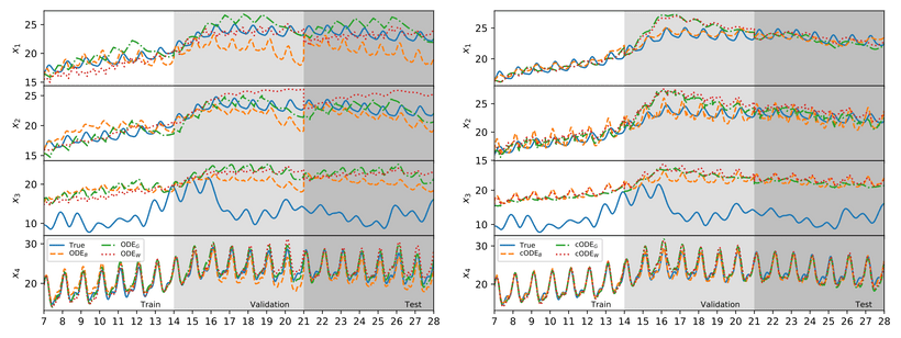
The traces presented above compare the predicted states of non-constrained and constrained models with the ground-truth system’s state trajectory. Non-constrained models exhibit noticable drift over time, especially when predicting states not observed in the training set. As one might expect from the results in Table 1, cODE_B tracks state variables most effectively, though all models struggle to track $x_3$ which is the least correlated with observed variable $x_4$ .

Conclusion

Our structured neural network architecture for modeling discrete ODEs demonstrates excellent generalization capability even in data-limited scenarios. The careful integration of prior knowledge about the physical behaviors of a system through algebraic structure and inequality constraints ensures both the sample efficiency and physical realism of the model. Model parameter eigenvalue regularization provides further stability guarantees to ensure the model’s efficacy and safety in real-world applications. The general structure of the model imbues it with enough flexibility to model physical systems with varying algebraic structure and dynamics.

To ease the implementation of structured neural ODE models for real-world engineering applications, we are developing a software library called NeuroMANCER to provide a host of physics-informed priors commonly encountered in engineering spaces. We hope that this library will empower engineers and researchers with the tools to build effective, stable dynamic system models.

Acknowledgements

This work was funded by the Mathematics for Artificial Reasoning in Science (MARS) investment at Pacific Northwest National Laboratory (PNNL).